For this tutorial, we will be using the coiaf package to estimate the complexity of infection (COI) from SNP barcode data. Instructions to install this package may be found here.
The data
coiaf expects a matrix of within sample reference allele frequencies (WSAF), as well as an estimate of population level reference allele frequencies (PLAF). The WSAF matrix should have samples in rows and sites in columns. The PLAF should be a vector of length equal to the number of sites. To explore this, we will use simulated SNP barcoding data as described here. We will load the data using the vcfR package.
Scanning file to determine attributes.
File attributes:
  meta lines: 76
  header_line: 77
  variant count: 100
  column count: 109

Meta line 76 read in.
All meta lines processed.
gt matrix initialized.
Character matrix gt created.
  Character matrix gt rows: 100
  Character matrix gt cols: 109
  skip: 0
  nrows: 100
  row_num: 0

Processed variant: 100
All variants processed
To calculate within host allele frequencies, we need to extract the depth of coverage and allele counts
coverage <-t(vcfR::extract.gt(vcf_data, element ="DP", as.numeric =TRUE))counts_raw <-t(vcfR::extract.gt(vcf_data, element ="AD"))counts <- vcfR::masplit( counts_raw, record =1, sort =FALSE, decreasing =FALSE)# We then directly calculate the WSAFwsaf <- counts / coverage# and estimate the PLAF with the empirical mean across samplesplaf <-colMeans(wsaf, na.rm =TRUE)
Running coiaf
coiaf calcualtes the COI on a sample by sample basis, so we need to break up the WSAF matrix into a list of data frames
We can then run coiaf on each sample using purrr::map_dbl
results <- purrr::map_dbl( input_data, ~ coiaf::optimize_coi(.x, data_type ="real"))# We can then combine the results into a data frame with the sample namesres_df <-data.frame(Patient =rownames(wsaf), COI = results)
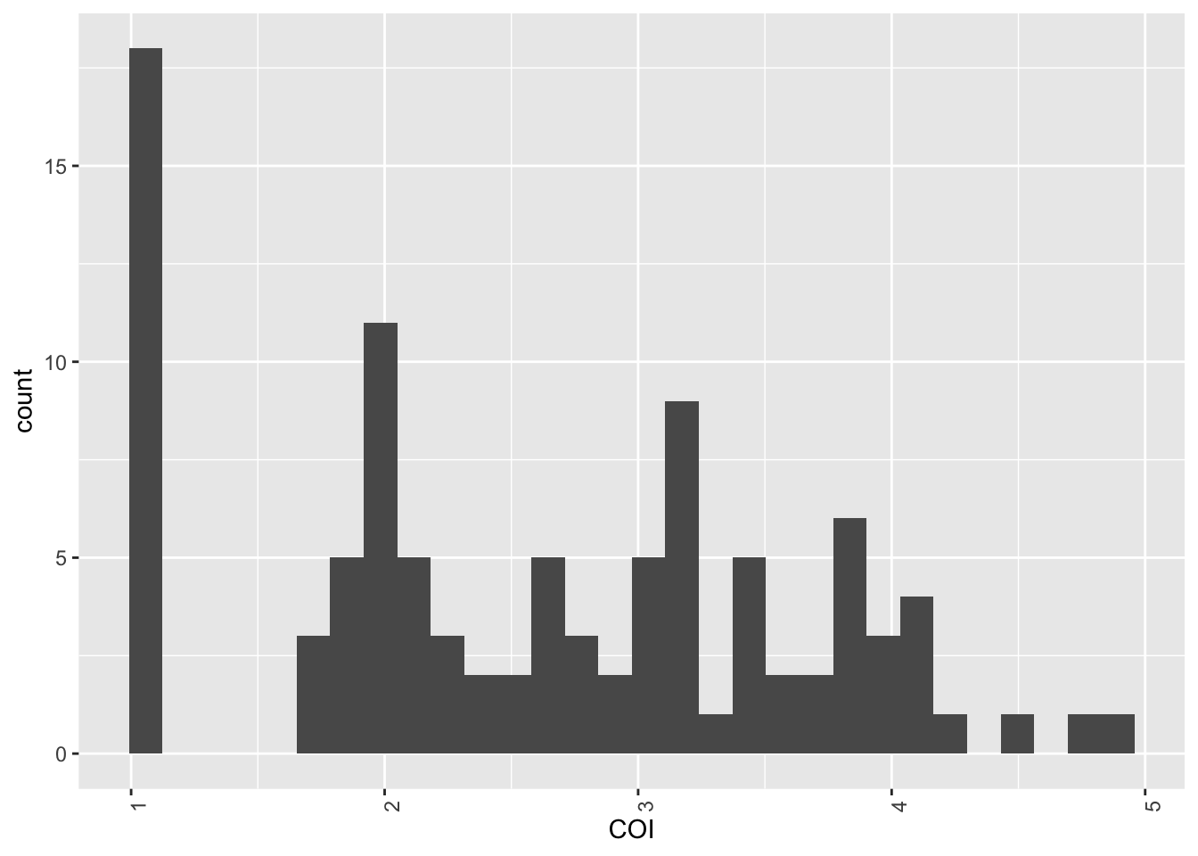
Plotting the results
Now that we have the estimated COI for each sample, we can plot the results.
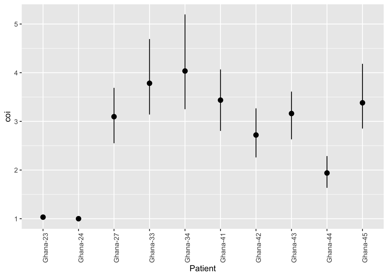
coiaf also provides a function to estimate the uncertainty in the COI estimate. This function uses a non-parametric bootstrap to estimate the uncertainty in the COI estimate. Note that this function can take a long time to run, so we will only run it on the first 10 samples.
# We can use the same input data as beforebootstrap_results <- purrr::map( input_data[1:10], ~ coiaf::bootstrap_ci(.x, solution_method ="continuous"))
[1] "All values of t are equal to 1 \n Cannot calculate confidence intervals"
# We can then combine the results into a data frame with the sample namesbootstrap_df <-data.frame(Patient =rownames(wsaf)[1:10], bootstrap_results |> dplyr::bind_rows())
In this tutorial, we have shown how to use coiaf to estimate the complexity of infection from SNP barcode data. For more information on the package, please see the package documentation.