Fitting odin2 models to data

WARNING: The concepts here are stable, but some of the interface will change, in particular function names.

With a dynamical model we can simulate forwards in time and see how a system might change over time, given a set of parameters. If we have a time series data set though, we can go a step further and find parameters consistent with the data. This vignette gives an introduction to the approaches to fitting to data available for odin2 models. This support largely derives from the monty and dust2 packages and we will refer the reader to their documentation where further detail is on offer.

Setting the scene

We’ll start with a simple data set of daily cases of some disease over time

data <- read.csv("incidence.csv")
head(data)
#>   cases time
#> 1     3    1
#> 2     2    2
#> 3     2    3
#> 4     2    4
#> 5     1    5
#> 6     3    6
plot(cases ~ time, data, pch = 19, las = 1,
     xlab = "Time (days)", ylab = "Cases")

The data here shows a classic epidemic, with cases rising up to some peak and falling. We will try fitting this with a simple compartmental SIR (Susceptible-Infected-Recovered) model, which we will write here in odin2. There are a number of possible ways of writing this, but here we’ll go for a stochastic discrete-time version, mostly because it will allow us to demonstrate a number of features of odin2, dust2 and monty (and because the ODE version is not yet written).

Before fitting the data, we’ll write out a model that captures the core ideas (this is replicated from vignette("odin2"))

sir <- odin2::odin({
  initial(S) <- N - I0
  initial(I) <- I0
  initial(R) <- 0
  initial(incidence) <- 0
  update(S) <- S - n_SI
  update(I) <- I + n_SI - n_IR
  update(R) <- R + n_IR
  update(incidence) <- if (time %% 1 == 0) n_SI else incidence + n_SI
  n_SI <- Binomial(S, p_SI)
  n_IR <- Binomial(I, p_IR)
  p_SI <- 1 - exp(-beta * I / N * dt)
  p_IR <- 1 - exp(-gamma * dt)
  beta <- parameter()
  gamma <- parameter()
  I0 <- parameter()
  N <- 1000
}, quiet = TRUE)

We can initialise this system and simulate it out over this time series and plot the results against the data:

pars <- list(beta = 0.3, gamma = 0.1, I0 = 5)
sys <- dust2::dust_system_create(sir(), pars, n_particles = 20, dt = 0.25)
dust2::dust_system_set_state_initial(sys)
time <- 0:100
y <- dust2::dust_system_simulate(sys, time)

The dust2::dust_system_simulate function returns an n_state by n_particle by n_time matrix (here, 4 x 20 x 101). We’re interested in incidence (the fourth row here), and extracting that gives us a 20 x 101 matrix, which we’ll transpose in order to plot it:

matplot(time, t(y[4, , ]), type = "l", lty = 1, col = "#00000055",
        xlab = "Time (days)", ylab = "Cases", las = 1)
points(cases ~ time, data, pch = 19, col = "red")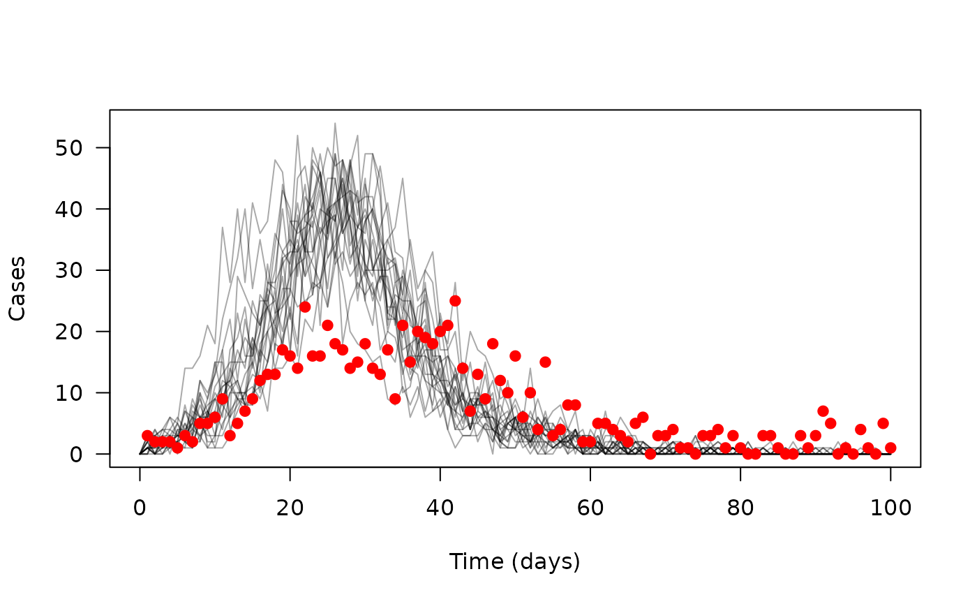

The modelled trajectories are in grey, with the data points overlaid in red – we’re not doing a great job here of capturing the data.

Comparing to data

We’re interested in fitting this model to data, and the first thing we need is a measure of goodness of fit, which we can also code into the odin model, but first we’ll explain the idea.

Our system moves forward in time until it finds a new data point; at this point in time we will have one or several particles present. We then ask for each particle how likely this data point is. This means that these calculations are per-particle and per-data-point.

Here, we’ll use a Poisson to ask “what is the probability of observing this many cases with a mean equal to our modelled number of daily cases”.

The syntax for this looks a bit different to the odin code above:

sir <- odin2::odin({
  initial(S) <- N - I0
  initial(I) <- I0
  initial(R) <- 0
  initial(incidence) <- 0
  update(S) <- S - n_SI
  update(I) <- I + n_SI - n_IR
  update(R) <- R + n_IR
  update(incidence) <- if (time %% 1 == 0) n_SI else incidence + n_SI
  n_SI <- Binomial(S, p_SI)
  n_IR <- Binomial(I, p_IR)
  p_SI <- 1 - exp(-beta * I / N * dt)
  p_IR <- 1 - exp(-gamma * dt)
  beta <- parameter()
  gamma <- parameter()
  I0 <- parameter()
  N <- 1000

  # Comparison to data
  cases <- data()
  cases ~ Poisson(incidence)
}, quiet = TRUE)

These last two lines are the new addition to the odin code. The first says that cases will be found in the data. The second restates our aim from the previous paragraph, comparing the observed cases against modelled incidence. The syntax here is designed to echo that of the monty DSL.

With this version of the model we can compute likelihoods with dust2’s machinery.

Stochastic likelihood with a particle filter

Our system is stochastic; each particle will produce a different trajectory and from that a different likelihood. Each time we run the system we get a different combination of likelihoods. We can use a particle filter to generate an estimate of the marginal likelihood, averaging over this stochasticity. This works by resampling the particles at each point along the time series, according to how likely they are.

filter <- dust2::dust_filter_create(sir(), 0, data, n_particles = 200)

Each time we run this filter the likelihood will be slightly (or very) different:

dust2::dust_likelihood_run(filter, pars)
#> [1] -276.5955
dust2::dust_likelihood_run(filter, pars)
#> [1] -282.6044

If you run the filter enough times a distribution will emerge of course. Let’s compare two points in parameter space, varying the beta parameter and running the filter 100 times each:

pars1 <- modifyList(pars, list(beta = 0.25))
pars2 <- modifyList(pars, list(beta = 0.23))
ll1 <- replicate(100, dust2::dust_likelihood_run(filter, pars1))
ll2 <- replicate(100, dust2::dust_likelihood_run(filter, pars2))

xb <- seq(floor(min(ll1, ll2)), ceiling(max(ll1, ll2)), by = 1)
hist(ll2, breaks = xb, col = "#0000ff99", freq = FALSE,
     xlab = "Log likelihood", ylab = "Density", main = "")
hist(ll1, breaks = xb, add = TRUE, freq = FALSE, col = "#ff000099")
abline(v = c(mean(ll1), mean(ll2)), col = c("red", "blue"), lwd = 2)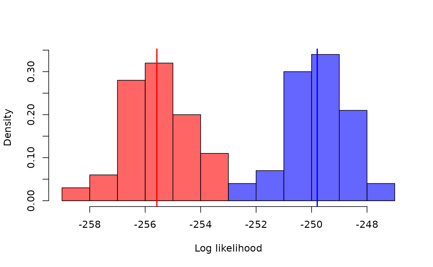

So even a relatively small difference in a parameter leads to a difference in the log-likelihood that is easily detectable in only 100 runs of the filter, even when the distributions overlap. However, it does make optimisation-based approaches to inference, such as maximum likelihood, tricky because it’s hard to know which way “up” is if each time you try a point it might return a different height.

If you run a particle filter with the argument save_history = TRUE then we save the trajectories of particles over time:

dust2::dust_likelihood_run(filter, list(beta = 0.2, gamma = 0.1), save_history = TRUE)
#> [1] -246.6374

You can access these with dust2::dust_likelihood_last_history():

h <- dust2::dust_likelihood_last_history(filter)

The result here is a 4 x 100 x 200 array:

dim(h)
#> [1]   4 200 100

The dimensions represent, in turn:

4 state variables
200 particles
100 time steps (corresponding to the data)

Considering just the fourth state, representing incidence, and plotting over time, you may be able to make out the tree structure of the trajectories, with fewer distinct traces at the start of the time series, and some traces more heavily represented in the final sample than others:

matplot(t(h[4, , ]), type = "l", lty = 1, col = "#00000022")
points(cases ~ time, data, pch = 19, col = "red")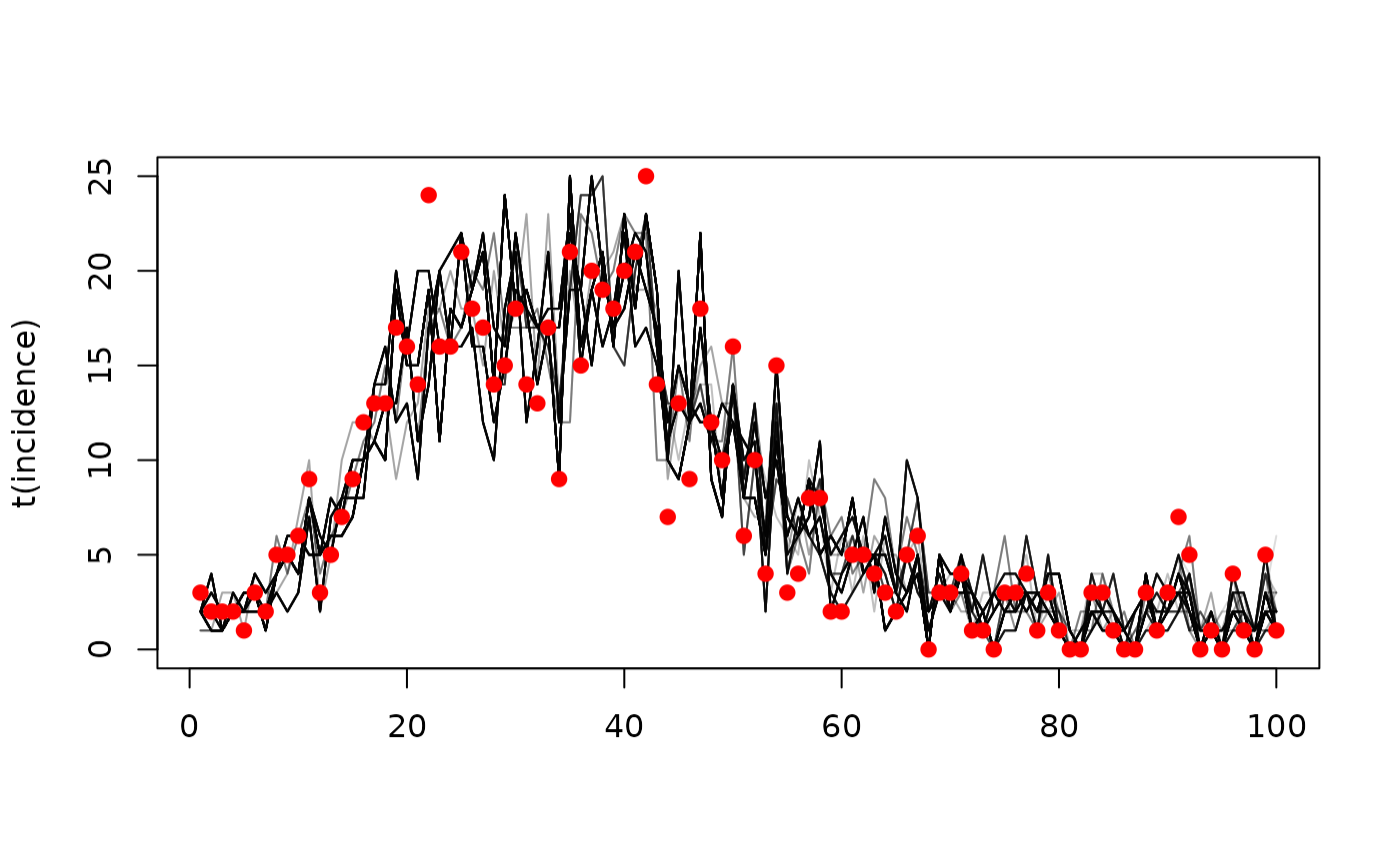

Inference with particle MCMC (pMCMC)

We can use MCMC to explore this model, but to do this we will need a prior. We’ll use monty’s DSL to create one; this looks similar to the odin code above:

prior <- monty::monty_dsl({
  beta ~ Exponential(mean = 0.3)
  gamma ~ Exponential(mean = 0.1)
})

Here we define a prior that covers beta and gamma, two of the three input parameters to our odin model. This prior is a monty_model object, which we can use to sample from, compute log densities with (to compute the prior), etc.

We also need to adapt our dust2 filter object above for use with monty. All we need to do here is to describe how a vector of statistical parameters (here beta and gamma) will be converted into the inputs that the sir system needs to run (here a list with elements beta, gamma and I0). We do this with a monty::monty_packer object:

sir_packer <- monty::monty_packer(c("beta", "gamma"), fixed = list(I0 = 5))

With this packer we can convert from a list of name-value pairs suitable for initialising a dust2 system into a vector of parameters suitable for use with monty:

sir_packer$pack(pars)
#> [1] 0.3 0.1

and we can carry out the inverse:

sir_packer$unpack(c(0.3, 0.1))
#> $beta
#> [1] 0.3
#> 
#> $gamma
#> [1] 0.1
#> 
#> $I0
#> [1] 5

Combining the filter and packer we create a monty model, which we’ll call likelihood, as that’s what it represents:

likelihood <- dust2::dust_likelihood_monty(filter, sir_packer)

This likelihood is now also a monty_model object:

likelihood
#> 
#> ── <monty_model> ───────────────────────────────────────────────────────────────
#> ℹ Model has 2 parameters: 'beta' and 'gamma'
#> ℹ This model:
#> • is stochastic
#> ℹ See `?monty_model()` for more information

The monty package provides a high-level interface for working with these objects. For example, to compute the likelihood we could now use monty::monty_model_density():

monty::monty_model_density(likelihood, c(0.2, 0.1))
#> [1] -244.9629

The difference to using dust2::dust_likelihood_run here is now we provide a parameter vector from our statistical model, rather than the inputs to the odin/dust model. This conforms to the interface that monty uses and lets us run things like MCMC.

We can combine the prior and the likelihood to create a posterior:

posterior <- prior + likelihood

The last ingredient required for running an MCMC is a sampler. We don’t have much choice with a model where the likelihood is stochastic, we’ll need to run a simple random walk. However, for this we still need a proposal matrix (the variance covariance matrix that is the parameter for a multivariate Gaussian - we’ll draw new positions from this). In an ideal world, this distribution will have a similar shape to the target distribution (the posterior) as this will help with mixing. To get started, we’ll use an uncorrelated random walk with each parameter having a fairly wide variance of 0.02

sampler <- monty::monty_sampler_random_walk(diag(2) * 0.02)

We can now run an MCMC for 100 samples

samples <- monty::monty_sample(posterior, sampler, 100,
                               initial = sir_packer$pack(pars))

We need to develop nice tools for working with the outputs of the sampler, but for now bear with some grubby base R manipulation.

The likelihood here is very “sticky”

plot(samples$density, type = "l")

It’s hard to say a great deal about the parameters beta (per-contact transmission rate) and gamma (recovery rate) from this few samples, especially as we have very few effective samples:

plot(t(drop(samples$pars)), pch = 19, col = "#00000055")

Effective sampling

There are several things we can do here to improve how this chain mixes

We can try and find a better proposal kernel.
We can increase the number of particles used in the filter. This will reduce the variance in the estimate of the marginal likelihood, which means that the random walk will be less confused by fluctuations in the surface it’s moving over. This comes at a computational cost though.
We can increase the number of threads (effectively CPU cores) that we are using while computing the likelihood. This will scale fairly efficiently through to at least 10 cores, with the likelihood calculations being almost embarrassingly parallel. This will help to offset some of the costs incurred above.
We can run multiple chains at once. We don’t yet have a good parallel runner implemented in monty but it is coming soon. This will reduce wall time (because each chain runs at the same time) and also allows us to compute convergence diagnostics which will reveal how well (or badly) we are doing.
We can try a deterministic model (see below) to get a sense of the general region of high probability space.

Here, we apply most of these suggestions at once, using a variance-covariance matrix that I prepared earlier:

filter <- dust2::dust_unfilter_create(sir(), 0, data, n_particles = 1000)
likelihood <- dust2::dust_likelihood_monty(filter, sir_packer)
vcv <- matrix(c(0.0005, 0.0003, 0.0003, 0.0003), 2, 2)
sampler <- monty::monty_sampler_random_walk(vcv)
samples <- monty::monty_sample(posterior, sampler, 1000,
                               initial = sir_packer$pack(pars))
#> Sampling  ■■■■■■■■                         |  24% ETA:  3s
#> Sampling  ■■■■■■■■■■■■■■■■■■■■■■■■         |  77% ETA:  1s
#> Sampling  ■■■■■■■■■■■■■■■■■■■■■■■■■■■■■■■  | 100% ETA:  0s

The likelihood now quickly rises up to a stable range and is clearly mixing:

plot(samples$density, type = "l")

The parameters beta (per-contact transmission rate) and gamma (recovery rate) are strongly correlated

plot(t(drop(samples$pars)), pch = 19, col = "#00000055")

Deterministic models from stochastic

Another way of fitting this model is to simply throw away the stochasticity. In the model above we have the lines

  n_SI <- Binomial(S, p_SI)
  n_IR <- Binomial(I, p_IR)

which are the stochastic portion of the model. Each time step we compute the number of individuals who make the transition from S to I and from I to R by sampling from the binomial distribution. We can replace these calls by their expectations (so effectively making n_SI = S * p_SI) by running the model in “deterministic” mode.

This simplification of the stochastic model can be seen as taking expectations of the underlying random process, but there’s no reason to expect that this represents the mean of the whole model ( $E[f(x)] \neq f(E[x])$ , at least generally).

We have found these simplifications useful:

They are not stochastic, so you can use adaptive MCMC or other more efficient algorithms
They are orders of magnitude faster, because instead of running 100s or thousands of particles per likelihood evaluation you just run one
The region of high probability density of the deterministic model is often within the (broader) region of high probability density of the stochastic model, so you can use these models to create reasonable starting parameter values for your chains
The signs and relative magnitudes of the covariances among parameters are often similar between the deterministic and stochastic model, so you can use the deterministic model to estimate a variance-covariance matrix for your stochastic model – though you will need to increase all quantities in it

Obviously, this approximation comes with costs though:

You no longer have integer valued quantities from the expectations of samples in your discrete distributions, so you have to think about fractional individuals
The model can no longer account for stochastic effects, e.g., at low population sizes. This can make the model overly rigid, and it may poorly account for observed patterns
The fixed dt approach is a first order Euler solver which offers few stability guarantees, and this will differ from a system of ODEs solved with a better ODE solver

To create a deterministic “filter” (currently, and temporarily called an “unfilter”), use dust_unfilter_create() in place of dust_filter_create. This will replace all calls to stochastic functions with their expectations at the point of call.

unfilter <- dust2::dust_unfilter_create(sir(), 0, data)

In contrast with filter, above, multiple calls to unfilter with the same parameter set yield the same result.

dust2::dust_likelihood_run(unfilter, pars)
#> [1] -543.8531
dust2::dust_likelihood_run(unfilter, pars)
#> [1] -543.8531

We can now proceed as before, reusing our packer, prior and sampler objects, which are still useable here:

likelihood_det <- dust2::dust_likelihood_monty(unfilter, sir_packer)
posterior_det <- prior + likelihood_det
samples_det <- monty::monty_sample(posterior_det, sampler, 1000,
                                   initial = sir_packer$pack(pars))

Here, you can see the 1000 samples from the deterministic model (in blue) overlaid on top of the samples from the stochastic model (in grey):

plot(t(drop(samples$pars)), pch = 19, col = "#00000033")
points(t(drop(samples_det$pars)), pch = 19, col = "#0000ff33")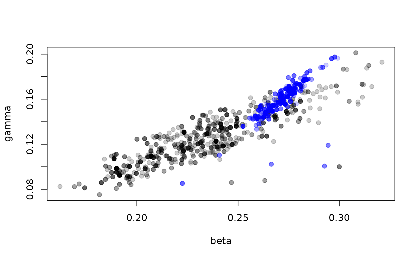

The estimated parameters here look overall shifted higher in the deterministic model, and the correlation between the parameters stronger. However, if we had no idea about what “good” parameters might be, this can get us into the approximately right location.

Differentiable models

We can go a step further than simply turning off stochasticity to create a deterministic model; now that we’ve got a deterministic likelihood function we can also differentiate that likelihood with respect to (some of) the parameters.

sir <- odin2::odin({
  initial(S) <- N - I0
  initial(I) <- I0
  initial(R) <- 0
  initial(incidence) <- 0
  update(S) <- S - n_SI
  update(I) <- I + n_SI - n_IR
  update(R) <- R + n_IR
  update(incidence) <- if (time %% 1 == 0) n_SI else incidence + n_SI
  n_SI <- Binomial(S, p_SI)
  n_IR <- Binomial(I, p_IR)
  p_SI <- 1 - exp(-beta * I / N * dt)
  p_IR <- 1 - exp(-gamma * dt)
  beta <- parameter(differentiate = TRUE)
  gamma <- parameter(differentiate = TRUE)
  I0 <- parameter()
  N <- 1000

  # Comparison to data
  cases <- data()
  cases ~ Poisson(incidence)
}, quiet = TRUE)

This the same model as above, except for the definition of beta and gamma, which now contain the argument derivative = TRUE.

This system can be used as a stochastic model (created via dust2::dust_filter_create) just as before. The only difference is where the model is created using dust2::dust_unfilter_create().

unfilter <- dust2::dust_unfilter_create(sir(), 0, data)

When you run the unfilter, you can now provide the argument adjoint = TRUE which will enable use of dust_likelihood_last_gradient() (we may make this the default in future).

dust2::dust_likelihood_run(unfilter, pars, adjoint = TRUE)
#> [1] -543.8531
dust2::dust_likelihood_last_gradient(unfilter)
#> [1] -6187.984  4780.146

We can create a monty model with this, as before:

likelihood <- dust2::dust_likelihood_monty(unfilter, sir_packer)
likelihood
#> 
#> ── <monty_model> ───────────────────────────────────────────────────────────────
#> ℹ Model has 2 parameters: 'beta' and 'gamma'
#> ℹ This model:
#> • can compute gradients
#> ℹ See `?monty_model()` for more information

and this model advertises that it can compute gradients now!

So from monty we can use monty::monty_model_density() and monty::monty_model_gradient() to compute log-likelihoods and gradients.

monty::monty_model_density(likelihood, c(0.2, 0.1))
#> [1] -375.0398
monty::monty_model_gradient(likelihood, c(0.2, 0.1))
#> [1]  5093.697 -2890.574

Because the prior contained gradient information, a posterior created with this version of the model also has gradients:

posterior <- likelihood + prior
posterior
#> 
#> ── <monty_model> ───────────────────────────────────────────────────────────────
#> ℹ Model has 2 parameters: 'beta' and 'gamma'
#> ℹ This model:
#> • can compute gradients
#> • can be directly sampled from
#> ℹ See `?monty_model()` for more information

With a model configured this way, you can use the Hamiltonian Monte Carlo method with monty::monty_sampler_hmc(), which can be far more efficient than a random walk once tuned.

WARNING”: Using derivative = TRUE on some parameters has the effect of making the rest use constant = TRUE. We will describe the effects of this in a vignette on differentiable models, soon.

Running multiple parameter sets at once

You can efficiently run multiple parameter sets at once; this will be parallelised where possible when enabled.

For dust2 systems

When initialising the dust system, you should:

pass a (typically unnamed) list of parameters, each element of which is a different set of parameters for the system
pass the n_groups argument indicating how many groups you wish to initialise

Here is a simple case with two parameter sets that differ in beta, each run with 20 particles:

pars2 <- list(list(beta = 0.3, gamma = 0.1, I0 = 5),
              list(beta = 0.2, gamma = 0.1, I0 = 5))
sys <- dust2::dust_system_create(sir(), pars2, n_particles = 20, n_groups = 2,
                                 dt = 0.25)
dust2::dust_system_set_state_initial(sys)
time <- 0:100
y <- dust2::dust_system_simulate(sys, time)

The dimensions of y is now

dim(y)
#> [1]   4  20   2 101

representing

4 state variables
20 particles
2 parameter groups
101 times

Consider just incidence as above:

matplot(time, t(y[4, , 1, ]), type = "l", lty = 1, col = "#ff000055",
        xlab = "Time (days)", ylab = "Cases", las = 1)
matlines(time, t(y[4, , 2, ]), type = "l", lty = 1, col = "#0000ff55")
points(cases ~ time, data, pch = 19)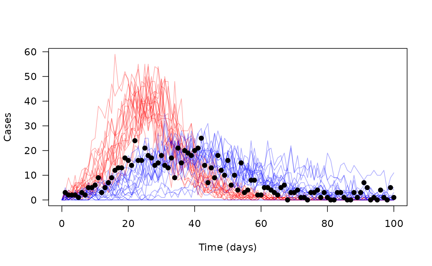

For dust2 filters/unfilters

Here we assume (require, really) that each parameter set is associated with a different data set. We may relax this in future, but this is the typical use case we have seen. We need an additional column called group in addition to time:

head(data2)
#>   group cases time
#> 1     1     3    1
#> 2     2     6    1
#> 3     1     2    2
#> 4     2     3    2
#> 5     1     2    3
#> 6     2     4    3

(this is just synthetic data for now, created by duplicating and perturbing the original data).

plot(cases ~ time, data2, subset = group == 2, pch = 19, col = "red",
     xlab = "Time (days)", ylab = "Cases")
points(cases ~ time, data2, subset = group == 1, pch = 19, col = "blue")

Because the data is grouped, we don’t need to tell dust2::dust_filter_create() that we have two groups, though you can pass n_groups = 2 here if you want, which will validate that you really do have exactly two groups in the data:

filter2 <- dust2::dust_filter_create(sir(), 0, data2, n_particles = 200)

When passing parameters into the filter, you now should mirror the format used in dust2::dust_system_run(); a list of lists:

dust2::dust_likelihood_run(filter2, pars2)
#> [1] -285.8723 -377.1315

We now have two likelihoods returned by the filter; one per group.

For the deterministic unfilter the process is the same:

unfilter2 <- dust2::dust_unfilter_create(sir(), 0, data2)
dust2::dust_likelihood_run(unfilter2, pars2)
#> [1] -543.8531 -621.4960

however, our gradient has picked up a dimension:

dust2::dust_likelihood_last_gradient(unfilter2)
#>           [,1]      [,2]
#> [1,] -6187.984  9986.701
#> [2,]  4780.146 -7449.405

Here, the first column is the gradient of the first parameter set, and the first row is the gradient of beta over parameter sets.

Compare with the single parameter case:

dust2::dust_likelihood_run(unfilter, pars2[[1]])
#> [1] -543.8531
dust2::dust_likelihood_last_gradient(unfilter)
#> [1] -6187.984  4780.146

For monty models

Here, rather than a parameter vector you would pass in a matrix, where each column represents a parameter set:

p <- cbind(c(0.2, 0.1), c(0.25, 0.1))

However, there’s a small bit of functionality we need to add here in dust2, still.

likelihood2 <- dust2::dust_likelihood_monty(filter2, sir_packer)
monty::monty_model_density(likelihood2, p)
#> [1] -245.587 -380.213