Sample from a model — monty

Sample from a model. Uses a Monte Carlo method (or possibly something else in future) to generate samples from your distribution. This is going to change a lot in future, as we add support for distributing over workers, and for things like parallel reproducible streams of random numbers. For now it just runs a single chain as a proof of concept.

Usage

monty_sample(
  model,
  sampler,
  n_steps,
  initial = NULL,
  n_chains = 1L,
  runner = NULL,
  restartable = FALSE,
  burnin = NULL,
  thinning_factor = NULL
)

Arguments

model: The model to sample from; this should be a monty_model for now, but we might change this in future to test to see if things match an interface rather than a particular class attribute.
sampler: A sampler to use. These will be described later, but we hope to make these reasonably easy to implement so that we can try out different sampling ideas. For now, the only sampler implemented is monty_sampler_random_walk().
n_steps: The number of steps to run the sampler for.
initial: Optionally, initial parameter values for the sampling. If not given, we sample from the model (or its prior). Alternatively, you can provide a monty_samples object here – the result of a previous call to this function – and we will sample some starting points from the final portion of the chains (the exact details here are subject to change, but we'll sample from the last 20 points or 5% of the chain, which ever smaller, with replacement, pooled across all chains in the previous sample).
n_chains: Number of chains to run. The default is to run a single chain, but you will likely want to run more.
runner: A runner for your chains. The default option is to run chains in series (via monty_runner_serial). The only other current option is monty_runner_parallel which uses the parallel package to run chains in parallel. If you only run one chain then this argument is best left alone.
restartable: Logical, indicating if the chains should be restartable. This will add additional data to the chains object.
burnin: Number of steps to discard as burnin. This affects only the recording of steps as your chains run; we don't record the first burnin steps. Generally you would want to do this in post-processing with monty_samples_thin() as this data is discarded with no chance of getting it back. However, if your observation process creates a large amount of data, then you may prefer to apply a burnin here to reduce how much memory is used.
thinning_factor: A thinning factor to apply while the chain is running. If given, then we save every thinning_factor'th step. So if thinning_factor = 2 we save every second step, and if 10, we'd save every 10th. Like burnin above, it is preferable to apply this in post processing with monty_samples_thin(). However, for slow-mixing chains that have a large observer output you can use this to reduce the memory usage. Use of thinning_factor requires that n_steps is an even multiple of thinning_factor; so if thinning_factor is 10, then n_steps must be a multiple of 10. This ensures that the last step is in the sample. The thinning factor cannot be changed when continuing a chain.

Value

A list of parameters and densities. We provide conversion to formats used by other packages, notably posterior::as_draws_array, posterior::as_draws_df and coda::as.mcmc.list; please let us know if you need conversion to something else. If you want to work directly with the output, the elements in the list include:

pars: An array with three dimensions representing (in turn) parameter, sample and chain, so that pars[i, j, k] is the ith parameter from the jth sample from the kth chain. The rows will be named with the names of the parameters, from your model.
density: A matrix of model log densities, with n_steps rows and n_chains columns.
initial: A record of the initial conditions, a matrix with as many rows as you have parameters and n_chains columns (this is the same format as the matrix form of the initial input parameter)
details: Additional details reported by the sampler; this will be a list of length n_chains (or NULL) and the details depend on the sampler. This one is subject to change.
observations: Additional details reported by the model. This one is also subject to change.

Examples

m <- monty_example("banana")
s <- monty_sampler_hmc(epsilon = 0.1, n_integration_steps = 10)
samples <- monty_sample(m, s, 2000)

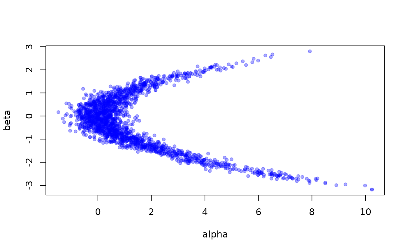
# Quick conversion of parameters into something plottable:
pars <- t(drop(samples$pars))
plot(pars, pch = 19, cex = 0.75, col = "#0000ff55")


# If you have the posterior package you might prefer converting to
# its format for performing diagnoses:
res <- posterior::as_draws_df(samples)
posterior::summarise_draws(res)
#> # A tibble: 2 × 10
#>   variable   mean median    sd   mad     q5   q95  rhat ess_bulk ess_tail
#>   <chr>     <dbl>  <dbl> <dbl> <dbl>  <dbl> <dbl> <dbl>    <dbl>    <dbl>
#> 1 alpha    1.08   0.587   1.71 0.934 -0.585  4.26  1.00    148.      92.6
#> 2 beta     0.0763 0.0436  1.03 0.962 -1.52   1.96  1.01     67.8     80.2

# At this point you could also use the 'bayesplot' package to plot
# diagnostics.