Load example models from monty. These models exist so that we can create (hopefully) interesting examples in the documentation without them becoming overwhelming. You should probably not use these for anything other than exploring the package.

Load small, ready-made target distributions for demonstrations, tests, and examples. These models exist so that we can create (hopefully) interesting examples in the documentation without them becoming overwhelming. All examples contain an analytic gradient and can thus be also used to explore gradient-based samplers such as monty_sampler_hmc.

Usage

monty_example(name, ...)

Arguments

name: Name of the example, as a string. See Details for supported models.
...: Optional parameters that are passed to create the model. All models can be created with no additional parameters, but you can tweak their behaviour by passing named parameters here. See Details.

Value

A monty_model object.

Supported models:

Each model has arguments that are passed through as ... in monty_example and are used to set up the example. This creates a monty_model object that will accept parameters, which are the values in the argument parameters passed to monty_model_density.

`banana`

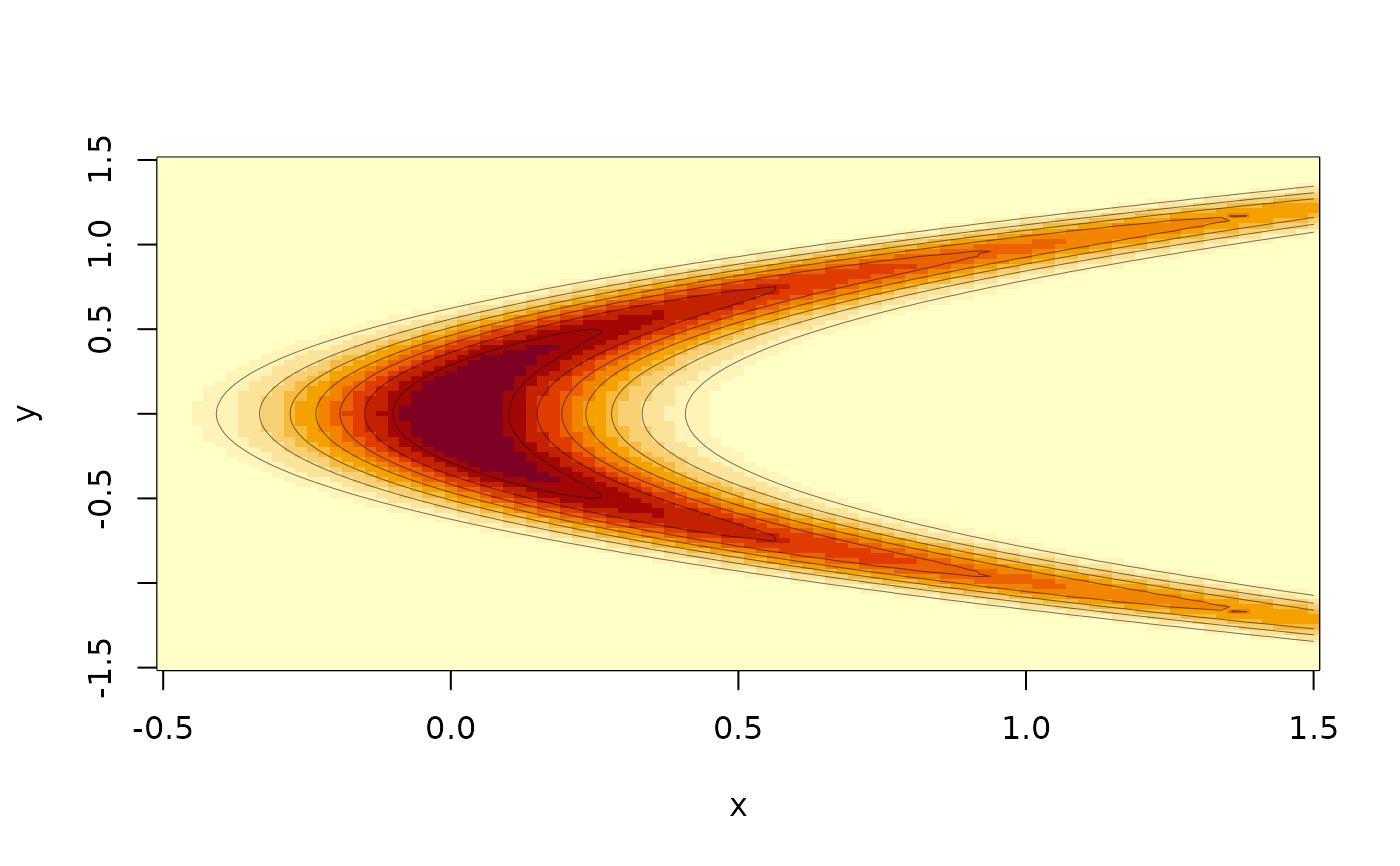
The banana model is a two-dimensional banana-shaped function, with strong local correlation. This example was picked because it is useful for illustrating the limitations of random-walk proposals. The model has two parameters alpha and beta and is based on two successive draws, one conditional on the other.

You can vary the argument sigma for this model on creation, the default is 0.5

`gaussian`

A multivariate Gaussian centred at the origin. Takes a variance-covariance-matrix as its argument. Parameters are letters a, b, ... up to the number of dimensions.

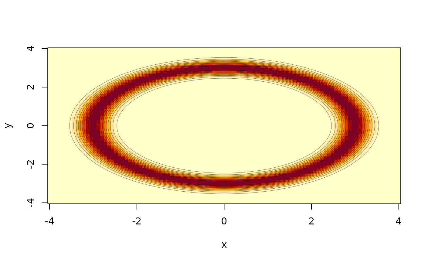
`ring`

A two-dimensional ring-shaped density whose log-density is proportional to $-(\|x\|-r)^2/(2\,sd^2)$. Includes an analytic gradient and a direct sampler in polar coordinates. The constructor takes that arguments r (default 3) and sd (default 0.2), and the parameters of the monty_model are x1 and x2 (corresponding to the two dimensions of the polar coordinates).

Increasing r or decreasing sd will make the ridge of high probability space narrower; this is easiest to visualise in true densities (rather than log density).

`mixture2d`

An equal-weight mixture of k isotropic 2D Gaussians with standard deviation sd and centres either provided by the argument (means) or drawn uniformly in a square of half-width spread (which must be provided if means is not provided). Includes an analytic gradient.

Examples

# Small helper function to make the plotting easier
show_2d_example <- function(m, rx, ry = rx, n = 101) {
  x <- seq(rx[[1]], rx[[2]], length.out = n)
  y <- seq(ry[[1]], ry[[2]], length.out = n)
  xy <- unname(t(as.matrix(expand.grid(x, y))))
  z <- exp(matrix(monty_model_density(m, xy), n, n))
  image(x, y, z)
  contour(x, y, z, add = TRUE, drawlabels = FALSE,
          lwd = 0.5, col = "#00000088")
}

# Banana target
m_banana <- monty_example("banana", sigma = 0.2)
show_2d_example(m_banana, c(-0.5, 1.5), c(-1.5, 1.5))


# Ring target with radius 3 and narrow thickness
m_ring <- monty_example("ring", r = 3, sd = 0.25)
show_2d_example(m_ring, c(-4, 4))


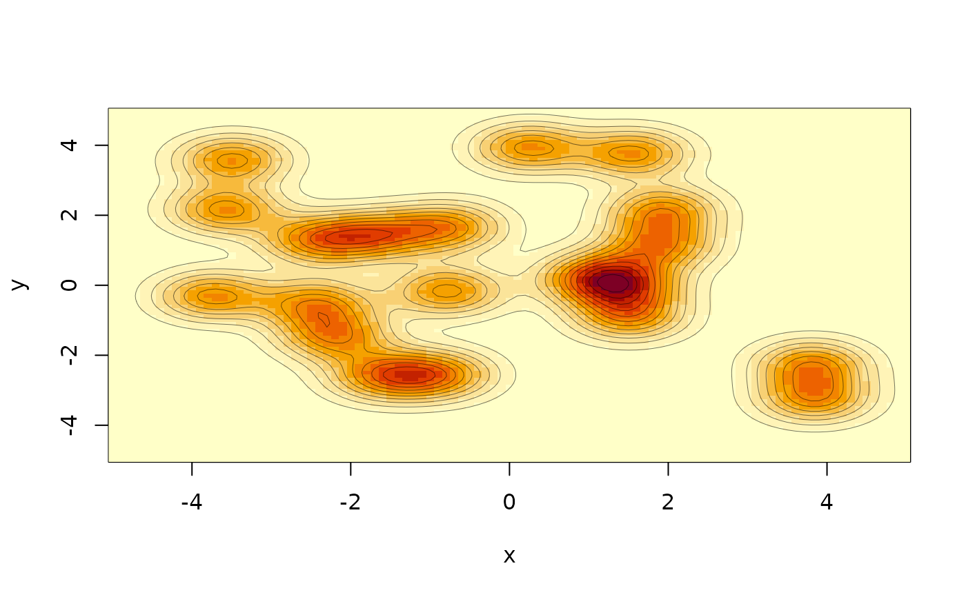
# 2D Gaussian mixture with 20 components
m_mixture <- monty_example("mixture2d", k = 20, sd = 0.5, spread = 4)
show_2d_example(m_mixture, c(-5, 5))