Introduction to monty • monty

This vignette is an introduction to some of the ideas in monty. Please note that the interface is not yet stable and some function names, arguments and ideas will change before the first generally usable version.

library(monty)

The basic idea

Draw samples from a model using Markov Chain Monte Carlo methods. To do this you will need:

A model: this is a monty_model() object and minimally knows about the names of its parameter vector (which is an unstructured real-valued vector) and can compute a log probability density. It may also be able to compute a gradient of this log density, or sample directly from parameter space (e.g., if it represents a prior distribution).
A sampler: this is some method of drawing samples from the model’s distribution in a sequence. We define several different sampler types, with the simplest one being monty_sampler_random_walk(), which implements a simple Metropolis algorithm random walk.
A runner: this controls how the chains will be run (e.g., one after another or in parallel).

The system is designed to be composable; you can work in a Bayesian way by defining a model representing a likelihood and another model representing a prior and then pick a sampler based on the capabilities of the model, and pick a runner based on the capabilities your computer.

The monty_model() interface is designed to be very flexible but not user-friendly. We expect to write a higher-level interface to help work with this, and describe how to write wrappers for models implemented in other packages (so you might write a model in dust or odin and an adaptor would make it easy to work with the tools provided by monty to start making inferences with your model).

An example

Before starting the example, it’s worth noting that there are far better tools out there to model this sort of thing (stan, bugs, jags, R itself - really anything). The aim of this section is to derive a simple model that may feel familiar. The strength of the package is when performing inference with custom models that can’t be expressed in these high level interfaces.

head(data)
#>     height   weight
#> 1 162.5401 45.92805
#> 2 159.9566 51.19368
#> 3 156.1808 44.56841
#> 4 168.4164 60.36933
#> 5 158.6978 52.14180
#> 6 154.7666 44.66696
plot(height ~ weight, data)

A simple likelihood, following the model formulation in “Statistical Rethinking” chapter 3; height is modelled as normally distributed departures from a linear relationship with weight.

fn <- function(a, b, sigma, data) {
  mu <- a + b * data$weight
  sum(dnorm(data$height, mu, sigma, log = TRUE))
}

We can wrap this density function in a monty_model. The data argument is “fixed” - it’s not part of the statistical model, so we’ll pass that in as the fixed argument:

likelihood <- monty_model_function(fn, fixed = list(data = data))
likelihood
#> 
#> ── <monty_model> ───────────────────────────────────────────────────────────────
#> ℹ Model has 3 parameters: 'a', 'b', and 'sigma'
#> ℹ See `?monty_model()` for more information

The prior we’ll make much nicer to work with in the future, but here we construct the density by hand as a sum of normally distributed priors on a and b, and a weak uniform prior on sigma.

prior <- monty_dsl({
  a ~ Normal(178, 100)
  b ~ Normal(0, 10)
  sigma ~ Uniform(0, 50)
})
prior
#> 
#> ── <monty_model> ───────────────────────────────────────────────────────────────
#> ℹ Model has 3 parameters: 'a', 'b', and 'sigma'
#> ℹ This model:
#> • can compute gradients
#> • can be directly sampled from
#> ℹ See `?monty_model()` for more information

The posterior distribution is the combination of these two models (indicated with a + because we’re adding on a log-scale, or because we are using prior and posterior; you can use monty_model_combine() if you prefer).

posterior <- likelihood + prior
posterior
#> 
#> ── <monty_model> ───────────────────────────────────────────────────────────────
#> ℹ Model has 3 parameters: 'a', 'b', and 'sigma'
#> ℹ This model:
#> • can be directly sampled from
#> ℹ See `?monty_model()` for more information

Constructing a sensible initial variance-covariance matrix is a bit of a trick, and using an adaptive sampler reduces the pain here. These values are chosen to be reasonable starting points.

vcv <- rbind(c(4.5, -0.088, 0.076),
             c(-0.088, 0.0018, -0.0015),
             c(0.076, -0.0015, 0.0640))
sampler <- monty_sampler_random_walk(vcv = vcv)

Now run the sampler. We’ve started from a good starting point to make this simple sampler converge quickly:

samples <- monty_sample(posterior, sampler, 2000, initial = c(114, 0.9, 3),
                        n_chains = 4)

We don’t aim to directly provide tools for visualising and working with samples, as this is well trodden ground in other packages. However, we can directly plot density over time:

matplot(samples$density, type = "l", lty = 1,
        xlab = "log posterior density", ylab = "sample", col = "#00000055")

And plots of our estimated parameters:

par(mfrow = c(1, 3))
plot(density(samples$pars["a", , ]), main = "a")
abline(v = 114, col = "red")
plot(density(samples$pars["b", , ]), main = "b")
abline(v = 0.9, col = "red")
plot(density(samples$pars["sigma", , ]), main = "sigma")
abline(v = 3, col = "red")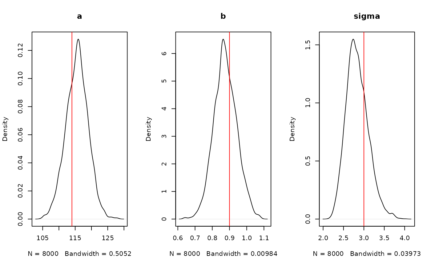

If you have coda installed you can convert these samples into a coda mcmc.list using coda::as.mcmc.list(), and if you have posterior installed you can convert into a draws_df using posterior::as_draws_df(), from which you can probably use your favourite plotting tools.

See vignette("samplers") for more information.