3 Stochasticity

Everybody get random

One of the key motivations for discrete time models is that they allow a natural mechanism for using stochasticity. By including stochasticity in our models we can better capture things like demographic effects where random fluctuations when population sizes are small have profound consequences for the longer term dynamics. In a deterministic system, things always happen the same way when you run them multiple times, but in a stochastic system – especially nonlinear ones – small changes in how the system arranges itself in its early steps can result in large changes in the dynamics later on, and this can help describe observed dynamics better.

3.1 Discrete-time

Stochastic models can be constructed in continuous-time. However, running realisations of such models is computationally expensive and becomes prohibitively so with increasing model complexity. Typically every time an event changes the state of the model (e.g. an infection or a recovery), the distribution of the time to the next event changes along with the probabilities governing the next event.

In odin we support discrete-time stochastic models as they are less expensive than continuous-time models as we just have to update the state of the model at a finite number of fixed time points. Models are updated at increments of dt, which currently must be the inverse of an integer (we recommend it be a non-recurring decimal, e.g. 1, 0.5, 0.25, 0.2, 0.125, 0.1 etc).

For the discrete-time stochastic models to be implemented in odin, they must follow the Markov property - given the entire history of the model up until time t, the distribution of the state at time t + dt must only depend upon the state of the model at time t.

Note

If you have used odin version 1, you will see that the interface for stochastic models has changed, and we no longer use functions named after R’s random functions. For example we now use Normal() rather than rnorm to refer to the normal distribution. See the odin2 migration vignette for more details.

library(odin2)
library(dust2)

3.2 A simple stochastic model

Here’s a simple SIR model, based on the one in Section 1.1, but which is stochastic:

sir <- odin({
  update(S) <- S - n_SI
  update(I) <- I + n_SI - n_IR
  update(R) <- R + n_IR
  update(incidence) <- incidence + n_SI

  p_SI <- 1 - exp(-beta * I / N * dt)
  p_IR <- 1 - exp(-gamma * dt)
  n_SI <- Binomial(S, p_SI)
  n_IR <- Binomial(I, p_IR)

  initial(S) <- N - I0
  initial(I) <- I0
  initial(R) <- 0
  initial(incidence, zero_every = 1) <- 0

  N <- parameter(1000)
  I0 <- parameter(10)
  beta <- parameter(0.2)
  gamma <- parameter(0.1)
})

This is a discrete-time model (using update() and not deriv()) as stochastic models must run in discrete time. We use dt to scale the rates, and adjusting dt will change the way that stochasticity affects the dynamics of the system.

The call to Binomial() samples from a binomial distribution, returning the number of successes from S (or I) draws, each with probability p_SI (or p_IR).

sir
#> 
#> ── <dust_system_generator: odin> ───────────────────────────────────────────────
#> ℹ This system runs in discrete time with a default dt of 1
#> ℹ This system has 4 parameters
#> → 'N', 'I0', 'beta', and 'gamma'
#> ℹ Use dust2::dust_system_create() (`?dust2::dust_system_create()`) to create a system with this generator
#> ℹ Use coef() (`?stats::coef()`) to get more information on parameters

The movement from S to I and from I to R are now drawn from a binomial distribution with probabilities that are computed from the rates (beta and gamma) multiplied by the change in time (dt). Some care is required to make sure that we subtract the same number of individuals from S as we add to I so we save this number as n_SI.

We can run this model just like before:

sys <- dust_system_create(sir, list())
dust_system_set_state_initial(sys)
t <- seq(0, 100)
y <- dust_system_simulate(sys, t)
y <- dust_unpack_state(sys, y)

Here is the number of infected individuals over time:

plot(t, y$I, type = "l", xlab = "Time", ylab = "Infected population")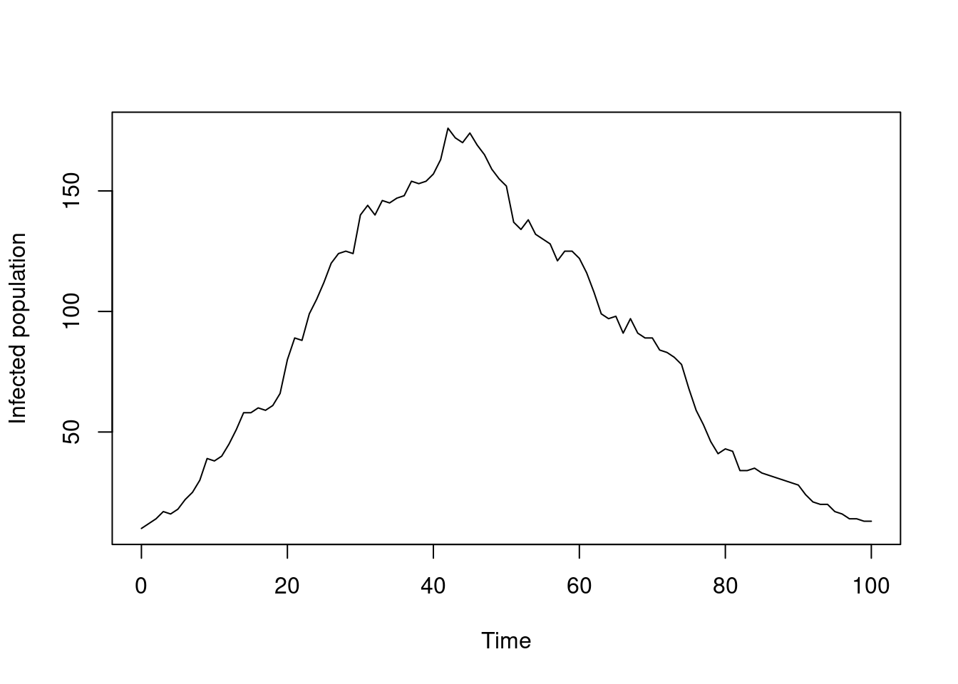

As in Section 1.1, we see an epidemic start, increase and then decay. Unlike the deterministic version though, the trajectory is not smooth, and it will be different each time we run it.

You can pass an argument n_particles when creating a system (the default is 1) to simulate multiple independent realisations at once:

sys <- dust_system_create(sir, list(), n_particles = 50)
dust_system_set_state_initial(sys)
y <- dust_system_simulate(sys, t)
y <- dust_unpack_state(sys, y)
matplot(t, t(y$I), type = "l", lty = 1, col = "#00000044",
        xlab = "Time", ylab = "Infected population")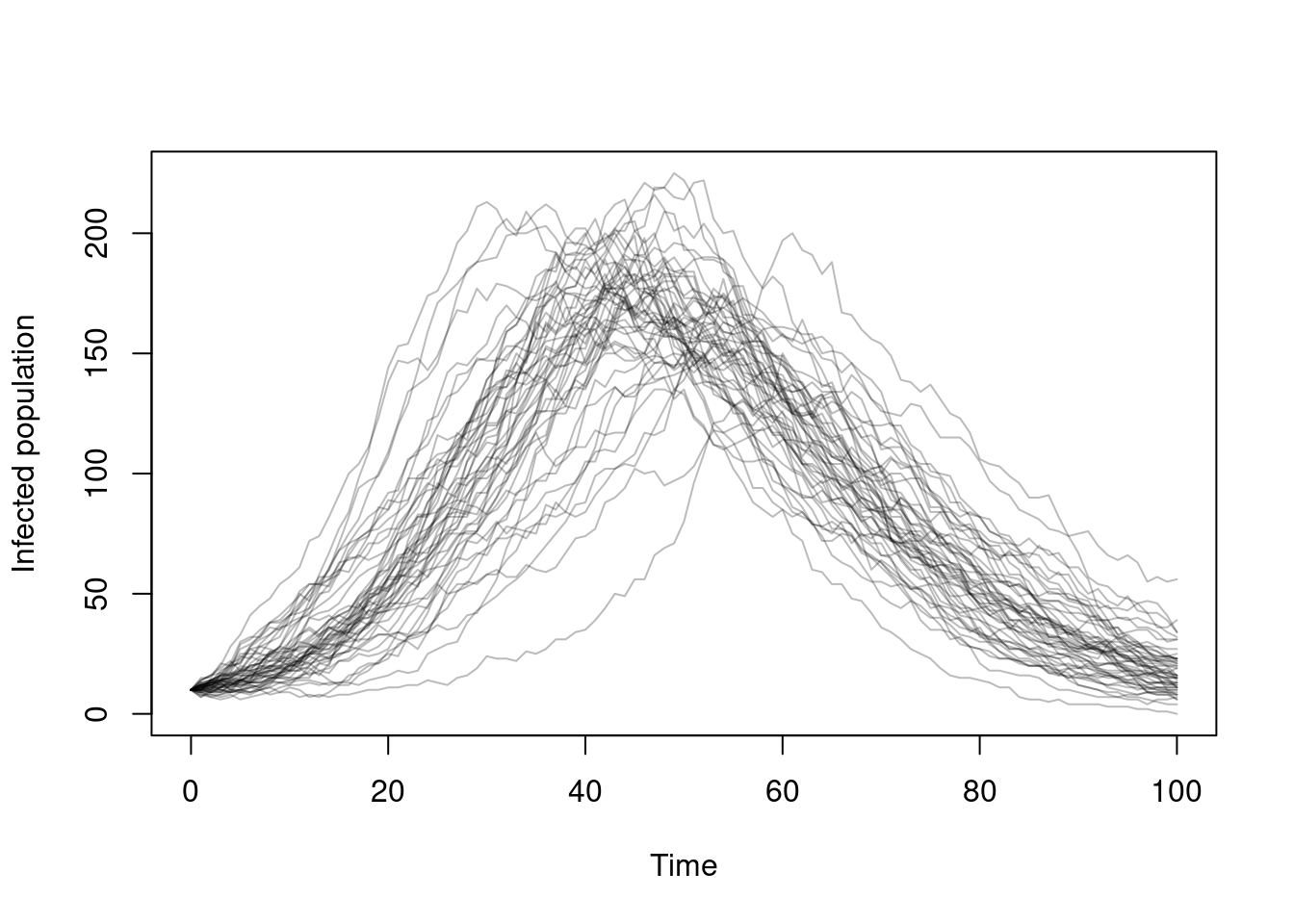

Here, we simulate 50 particles at once, all from the same point (10 individuals infected at time 0) and we see the similarities and differences in the trajectories: all follow approximately the same shape, and all rise and fall at approximately the same rate, but there is quite a bit of difference in the individual trajectories and the timings of when the epidemic peaks.

Note

The t() in plotting here moves time from the last dimension to the first, as is expected by matplot. We may write functions to help prepare output for plotting.

The stochastic effects will be stronger around the critical parameter values where the behaviour of the model diverges, or with smaller initial population sizes:

sys <- dust_system_create(sir, list(I0 = 5, gamma = 0.15), n_particles = 50)
dust_system_set_state_initial(sys)
y <- dust_system_simulate(sys, t)
y <- dust_unpack_state(sys, y)
matplot(t, t(y$I), type = "l", lty = 1, col = "#00000044",
        xlab = "Time", ylab = "Infected population")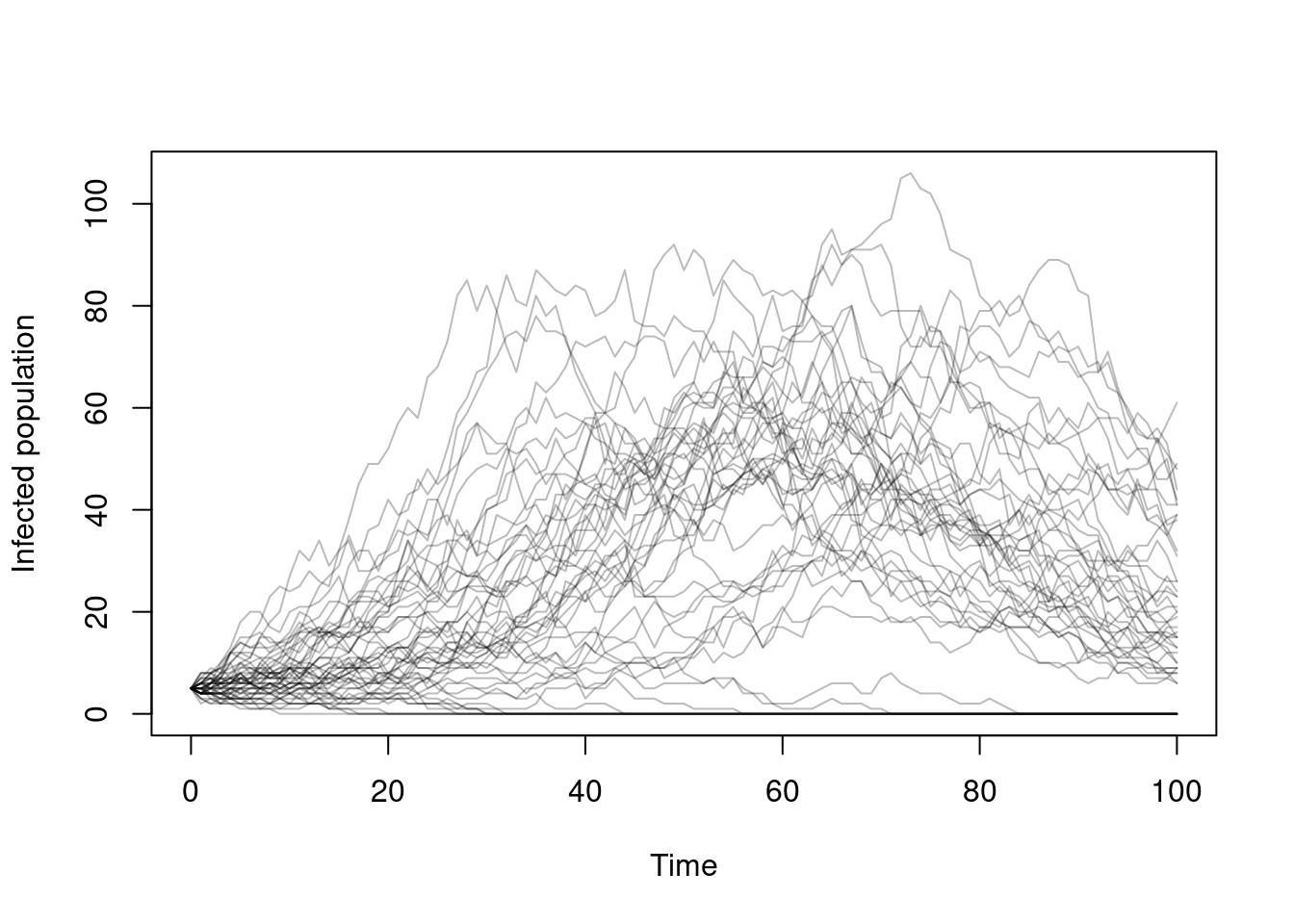

Here, we see some epidemics fail to take off, and a huge variation in where the peak is, with some trajectories only starting to take off at time 100 where in the previous example all were in decline.

We can see we have used zero_every to calculate the incidence of new infections in discrete-time in a similar way to how we did in the continuous-time deterministic model in Section 2.2.

Running the model we see the incidence produced:

pars <- list(beta = 1, gamma = 0.6)
sys <- dust_system_create(sir, pars, dt = 0.25)
dust_system_set_state_initial(sys)
t <- seq(0, 20, by = 0.25)
y <- dust_system_simulate(sys, t)
y <- dust_unpack_state(sys, y)
plot(t, y$incidence, type = "s", xlab = "Time", ylab = "Incidence")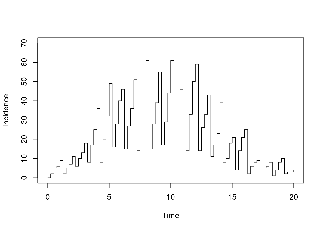

Our step is a quarter of a day, so we see four levels of incidence per day, with the last being the daily peak. Let’s run again, this time outputting only every day, we see:

sys <- dust_system_create(sir, pars, dt = 0.25)
dust_system_set_state_initial(sys)
t <- seq(0, 20)
y <- dust_system_simulate(sys, t)
y <- dust_unpack_state(sys, y)
plot(t, y$incidence, type = "p", xlab = "Time", ylab = "Incidence")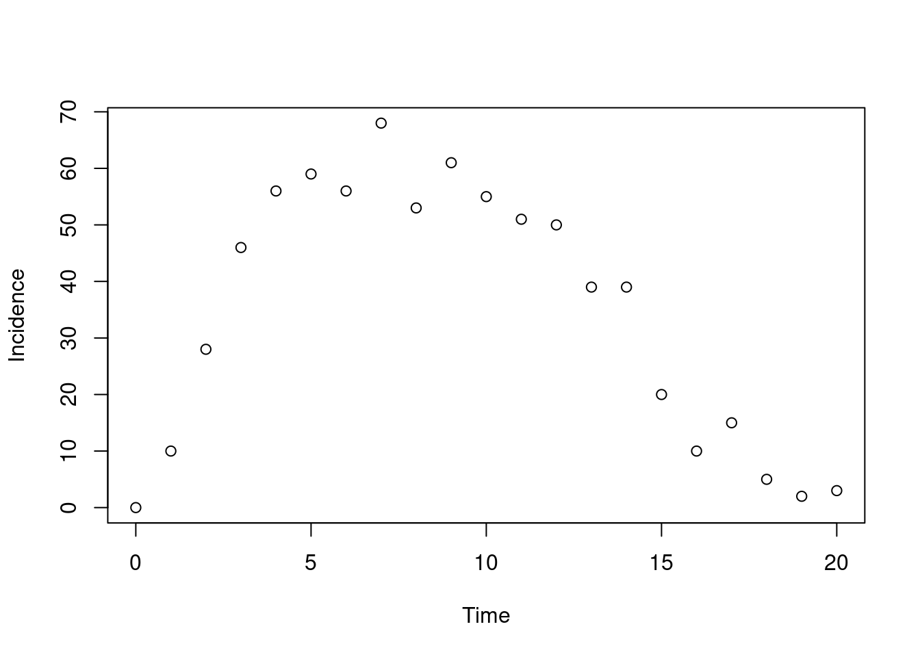

3.3 Supported random number functions

We have already seen use of Binomial draws, and we support other distributions. Support for the distributions includes both random draws and density calculations (more on that later). The support for these functions comes from monty and all the distributions are available for use in the both the odin DSL and the monty DSL (more on that also later).

Some distributions have several parametrisations; these are distinguished by the arguments to the functions. These distributions have a default parametrisation. For example, the Gamma distribution defaults to a shape and rate parametrisation so:

a <- Gamma(2, 0.1)
a <- Gamma(shape = 2, rate = 0.1)

draw from a Gamma distribution with a shape of 2 and a rate of 0.1, while

a <- Gamma(2, scale = 10)
a <- Gamma(shape = 2, scale = 10)

draw from a Gamma distribution with a shape of 2 and a scale of 10. You may find it is good practice to specify your arguments with such distributions whether using the default parameterisation or not.

Other supported distributions include the Normal, Uniform, Exponential, Beta and Poisson distributions. A full list of supported distributions and their parametrisations can be found here.

3.4 More sections to add:

Seeding
Something on threads and parallelism
Stochastic quantities vary over time