library(odin2)1 Getting started with odin
odin is a “Domain Specific Language” (DSL), that is a mini-language that is specifically tailored to a domain. By targeting a narrow domain we can have a language that expressively captures a problem and gives an efficient solution, as opposed to a general purpose language where you can write code that expresses anything, but your solution might either be quite verbose or have poor performance. You might be familiar with other DSLs such as the dplyr or ggplot2 syntax, or SQL if you have used databases.
1.1 A simple example
Here is a small system of differential equations for an “SIR” (Susceptible-Infected-Recovered) model:
\[\begin{gather*} \frac{dS}{dt} = -\beta S \frac{I}{N}\\ \frac{dI}{dt} = \beta S \frac{I}{N} - \gamma I\\ \frac{dR}{dt} = \gamma I \end{gather*}\]
And here is an implementation of these equations in odin:
sir <- odin({
  deriv(S) <- -beta * S * I / N
  deriv(I) <- beta * S * I / N - gamma * I
  deriv(R) <- gamma * I

  initial(S) <- N - I0
  initial(I) <- I0
  initial(R) <- 0

  N <- parameter(1000)
  I0 <- parameter(10)
  beta <- parameter(0.2)
  gamma <- parameter(0.1)
})
There are a few things to note here:
- equations are defined out of order; we just will things into existence and trust
odinto put them in the right order for us (much more on this later) - our system has “parameters”; these are things we’ll be able to change easily in it after creation
- every variable (as in, model variable — those that make up the state) has a pair of equations; an initial condition via
initial()and an equation for the derivative with respect to time viaderiv()
Note
Above you will see us struggle a bit with terminology, particularly between “system” and “model”. There are going to be two places where “model” can be usefully used - a model could be the generative model (here an SIR model) or it could be the statistical model, more the focus on the second half of the book. In order to make things slightly less ambiguous we will often refer to the generative model as a “system”, and this is reflected in the calls to functions in dust.
The odin() function will compile (more strictly, transpile) the odin code to C++ and then compile this into machine code and load it into your session. The resulting object is a dust_sytem_generator object:
sir
#>
#> ── <dust_system_generator: odin_system> ────────────────────────────────────────
#> ℹ This system runs in continuous time
#> ℹ This system has 4 parameters
#> → 'N', 'I0', 'beta', and 'gamma'
#> ℹ Use dust2::dust_system_create() (`?dust2::dust_system_create()`) to create a system with this generator
#> ℹ Use coef() (`?stats::coef()`) to get more information on parameters
As its name suggests, we can use this object to generate different versions of our system with different configurations. We pass this object to other functions from dust2 to create, run and examine our simulations.
1.2 Running systems using dust2
library(dust2)We create a system by using dust_system_create and passing in a list of parameters:
pars <- list()
sys <- dust_system_create(sir, pars)
sys
#>
#> ── <dust_system: odin_system> ──────────────────────────────────────────────────
#> ℹ single particle with 3 states
#> ℹ This system runs in continuous time
#> ℹ This system has 4 parameters that can be updated via `dust_system_update_pars`
#> → 'N', 'I0', 'beta', and 'gamma'
#> ℹ Use coef() (`?stats::coef()`) to get more information on parameters
To interact with a system, you will use functions from dust2, which we’ll show below.
All systems start off with a state of all zeros:
dust_system_state(sys)
#> [1] 0 0 0
There are two ways of setting state:
- Provide a new state vector and set it with
dust_system_set_state - Use the initial condition from the model itself (the expressions with
initial()on the left hand side)
Here, we’ll use the latter, and use the initial condition defined in the odin code:
dust_system_set_state_initial(sys)
dust_system_state(sys)
#> [1] 990  10   0
In general, the order of the state is arbitrary (though in practice it is fairly stable). To turn this state vector into something more interpretable you can use dust_unpack_state:
s <- dust_system_state(sys)
dust_unpack_state(sys, s)
#> $S
#> [1] 990
#>
#> $I
#> [1] 10
#>
#> $R
#> [1] 0
This gives a named list of numbers, which means we can work with the output of the model in a more reasonable way.
Next, we want to run the system. There are two main functions for doing this:
dust_system_run_to_timewhich runs the system up to some point in time, but returns nothingdust_system_simulatewhich runs the system over a series of points in time and returns the state at these points in time
Here we’ll do the latter as it will produce something we can look at!
t <- seq(0, 150, by = 0.25)
y <- dust_system_simulate(sys, t)
dim(y)
#> [1]   3 601
This produces a 3 x 601 matrix. This is typical of how time-series data are produced from odin2/dust2 and may be a surprise:
- state will always be on the first dimension
- time will always be on the last dimension
This may take some getting used to at first, but practically some degree of manipulation will be required in any case if you want to plot things.
We’ll explore some other ways of plotting later, but here’s the number of individuals in the infectious class over time, as the epidemic proceeds.
plot(t, dust_unpack_state(sys, y)$I, type = "l",
     xlab = "Time", ylab = "Infected population")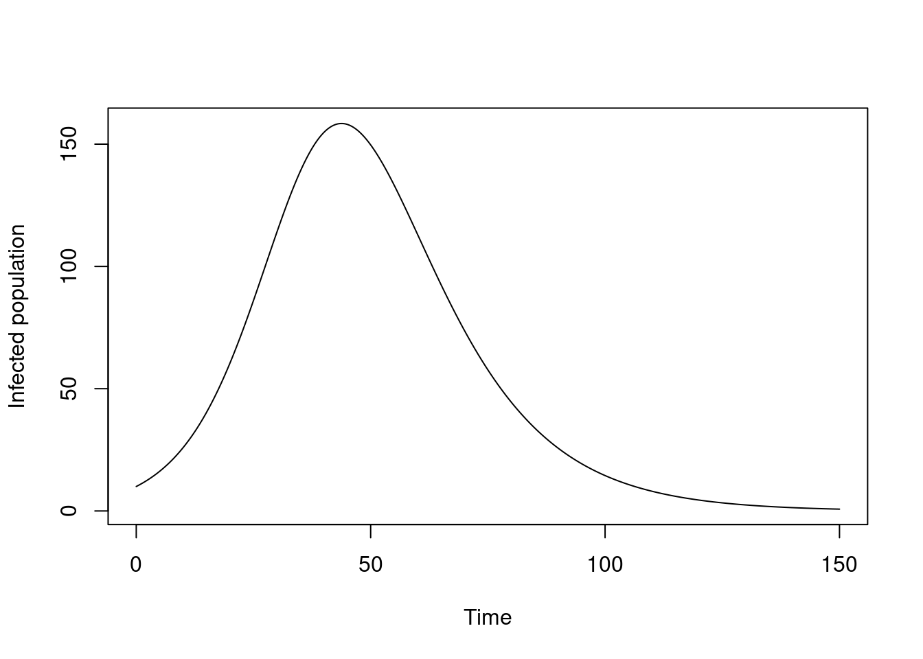
Once a system has been run to a time, you’ll need to reset it to run it again. For example, this won’t work
dust_system_simulate(sys, t)
#> Error:
#> ! Expected 'time[1]' (0) to be larger than the previous value (150)
The error here is trying to tell us that the first time in our vector t, which is 0, is smaller than the current time in the system, which is 150. We can query the system to get its current time, too:
dust_system_time(sys)
#> [1] 150
You can reset the time back to zero (or any other time) using dust_system_set_time:
dust_system_set_time(sys, 0)this does not reset the state, however:
dust_system_state(sys)
#> [1] 200.2910254   0.7422209 798.9667537
We can set new parameters, perhaps, and then update the state:
dust_system_update_pars(sys, list(I0 = 5))
dust_system_set_state_initial(sys)
dust_system_state(sys)
#> [1] 995   5   0
1.3 Going further
These are the lowest-level functions you would typically use, and we expect that you would combine these together yourself to perform specific tasks. For example suppose you wanted to explore how beta affected the epidemic trajectory over this set of times, we might write:
run_with_beta <- function(beta, t) {
  sys <- dust_system_create(sir, list(beta = beta))
  dust_system_set_state_initial(sys)
  idx <- dust_unpack_index(sys)$I
  drop(dust_system_simulate(sys, t, index_state = idx))
}
Here, we’ve used dust_unpack_index to get the index of the I compartment and passed that in as the index to dust_system_simulate.
We could then run this over a series of beta values:
beta <- seq(0.1, 0.3, by = 0.02)
y <- vapply(beta, run_with_beta, t, FUN.VALUE = numeric(length(t)))
matplot(t, y, type = "l", lty = 1, col = "steelblue4",
        xlab = "Time", ylab = "Infected population")
We could modify this to take a single system object and reset it each time (which might be useful if our model was slow to initialise). Alternatively we could simulate the whole grid of beta values at once:
pars <- lapply(beta, function(b) list(beta = b))
sys <- dust_system_create(sir, pars, n_groups = length(pars))
dust_system_set_state_initial(sys)
idx <- dust_unpack_index(sys)$I
y <- dust_system_simulate(sys, t, index_state = idx)
matplot(t, t(y[1, , ]), type = "l", lty = 1, col = "steelblue4",
        xlab = "Time", ylab = "Infected population")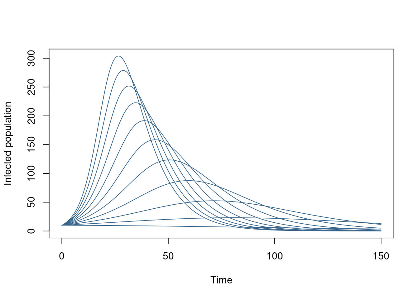
Or perhaps you would want to combine these approaches and start the simulation from a range of stochastic starting points. Given the unbounded range of things people want to do with dynamical models, the hope is that you can use the functions in dust2 in order to build workflows that match your needs, and that these functions should be well documented and efficient.