6  Looking back in time

Sometimes you want to look back in time as your system runs. We’ve already seen a simple case of this in Section 2.2, where we compute incidence from cumulative traces using zero_every. However, sometimes this is not enough:

• We might want a continuous incidence measure, such as the number of cases over the last n days
• You might want to respond to the state of your system further back in the past than one day

We can do this using delay differential equations (DDEs), in which rather than writing a system where \(dy/dt\) is expressed in terms of \(t\) and \(y(t)\), it also depends on \(y(t - \tau)\) where \(\tau\) is some fixed period back in time.

In general solving DDEs is hard, but if our main aim is to simply observe the behaviour over some interval they are fairly well behaved, empirically at least.

library(dust2)
library(odin2)

6.1 Calculating incidence, revisited

Here is the SIR model from Section 2.2, but here we’ve made some changes to compute incidence in continuous time too:

sir <- odin({
  deriv(S) <- -beta * S * I / N
  deriv(I) <- beta * S * I / N - gamma * I
  deriv(R) <- gamma * I
  rate_infections <- beta * S * I / N
  deriv(incidence) <- rate_infections
  deriv(infections) <- rate_infections

  initial(S) <- N - I0
  initial(I) <- I0
  initial(R) <- 0
  initial(incidence, zero_every = 1) <- 0
  initial(infections) <- 0

  N <- parameter(1000)
  I0 <- parameter(10)
  beta <- parameter(0.2)
  gamma <- parameter(0.1)

  infections_prev <- delay(infections, 1)
  output(incidence_continuous) <- infections - infections_prev
})

• We store the rate of infections rate_infections and we add a cumulative variable infections; the calculations for incidence are unchanged from before
• We compute the previous infections as the current cumulative infections delayed by one time unit
• We can then compute (and output) our continuous incidence measure as the difference between the current and previous cumulative infections

t <- seq(0, 20, by = 0.01)
sys <- dust_system_create(sir, list(beta = 1, gamma = 0.5))
dust_system_set_state_initial(sys)
y <- dust_system_simulate(sys, t)
y <- dust_unpack_state(sys, y)

Plotting the continuous measure (black) against our saw-toothed reset-every approach shows they line up at each time unit, but the black line changes smoothly while the red line shows increases followed by being reset.

plot(t, y$incidence_continuous, type = "l")
lines(t, y$incidence, type = "S", col = "red")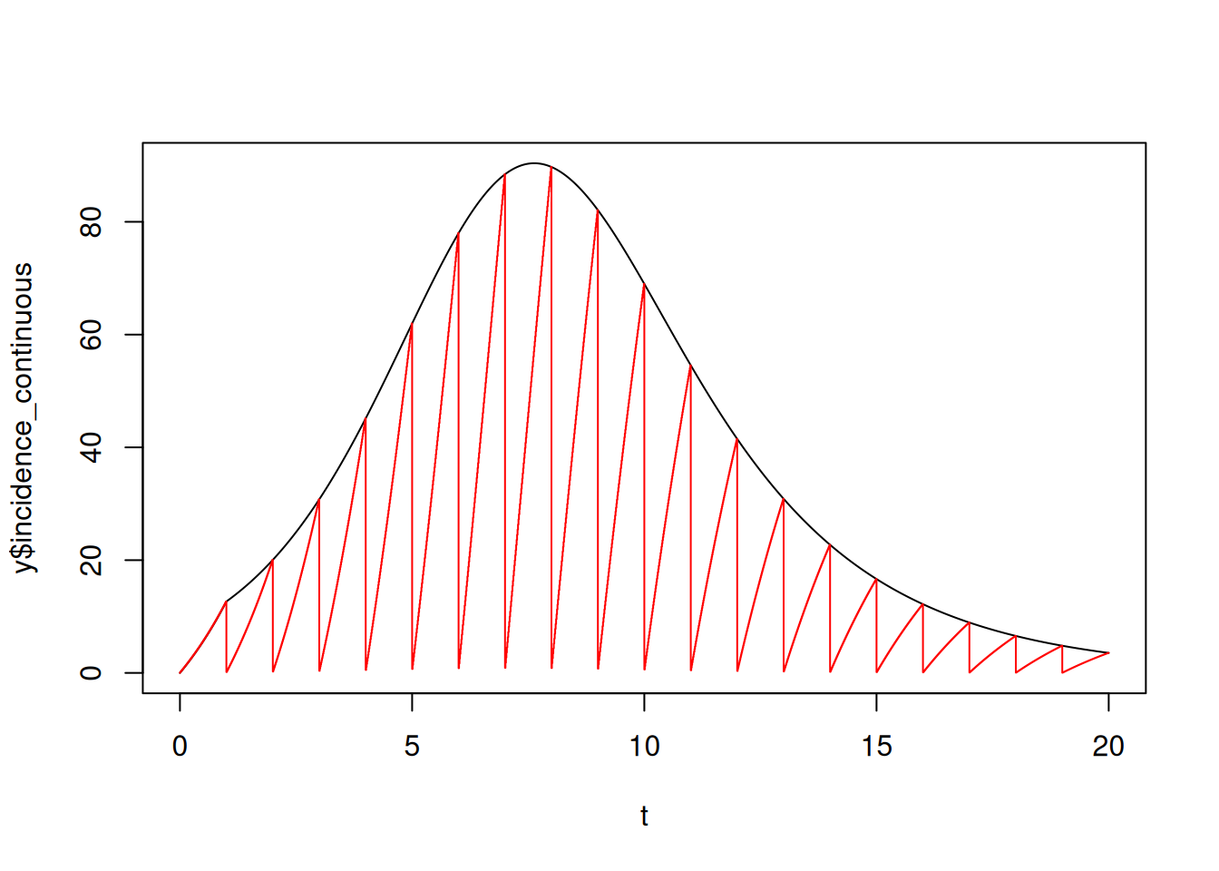

Note how the continuous incidence measure at between time 0 and 1 is inaccurate; this is because it is subtracting from the assumed cumulative infection value of zero before the simulation starts.

Without using delays, we have no smooth and continuous measure of incidence that we can use throughout the simulation.

6.2 Potential issues

Where your solution changes state abruptly, the handling of delays will be incorrect. Handling this correctly is non-trivial as it involves propagating all the harmonics of the points of change forward in time (that is, each change leaves an echo forward in time!). There are sophisticated solvers that can handle this, but we have not implemented one in dust2.

Delayed variables cannot be used everywhere; in particular they are not yet supported in comparison functions (this is on the radar), nor in events (which are not yet described in this book).