Deterministic models

Stochastic models are slow! Ignoring issues of parallelism and fast random numbers (see vignette("design")), you still must run the model some number of times within a particle filter to estimate the likelihood. We’re experimenting with alternative approaches to approximate the likelihood, including running the stochastic models “deterministically” with a single particle. In this case calls to rbinom(n, p) (for example) will be replaced with their mean (n * p). This is not exactly the same model as the stochastic model, nor is it directly even a limit case of it. However, we hope that it still lands in about the right area of high probability density and can be used for a pilot run before running a pmcmc properly.

We demonstrate this, as in vignette("sir_models") with our simple SIR model.

sir <- dust::dust_example("sir")

The data set is included within the package:

incidence <- read.csv(system.file("sir_incidence.csv", package = "mcstate"))
dt <- 0.25
data <- mcstate::particle_filter_data(incidence, time = "day", rate = 1 / dt)
#> Warning in mcstate::particle_filter_data(incidence, time = "day", rate = 1/dt):
#> 'initial_time' should be provided. I'm assuming '0' which is one time unit
#> before the first time in your data (1), but this might not be appropriate. This
#> will become an error in a future version of mcstate

A comparison function

compare <- function(state, observed, pars = NULL) {
  if (is.na(observed$cases)) {
    return(NULL)
  }
  exp_noise <- 1e6
  incidence_modelled <- state[1, , drop = TRUE]
  incidence_observed <- observed$cases
  lambda <- incidence_modelled +
    rexp(n = length(incidence_modelled), rate = exp_noise)
  dpois(x = incidence_observed, lambda = lambda, log = TRUE)
}

An index function for filtering the run state

index <- function(info) {
  list(run = 5L, state = 1:5)
}

Parameter information for the pMCMC, including a roughly tuned kernel so that we get adequate mixing

proposal_kernel <- rbind(c(0.00057, 0.00034), c(0.00034, 0.00026))
pars <- mcstate::pmcmc_parameters$new(
  list(mcstate::pmcmc_parameter("beta", 0.2, min = 0, max = 1,
                                prior = function(p) log(1e-10)),
       mcstate::pmcmc_parameter("gamma", 0.1, min = 0, max = 1,
                                prior = function(p) log(1e-10))),
  proposal = proposal_kernel)

First, run a stochastic fit, as in vignette("sir_models"). Increasing the number of particles will reduce the variance in the estimate of the the likelihood:

n_steps <- 300
n_particles <- 500

control <- mcstate::pmcmc_control(n_steps)
p1 <- mcstate::particle_filter$new(data, sir, n_particles, compare,
                                   index = index,
                                   n_threads = dust::dust_openmp_threads())
res1 <- mcstate::pmcmc(pars, p1, control = control)

then again, with the deterministic filter. The only change is to use the object mcstate::particle_deterministic and omit the n_particles element to the constructor (there will only ever be one particle!) and the n_threads element which has no effect here.

p2 <- mcstate::particle_deterministic$new(data, sir, compare, index = index)
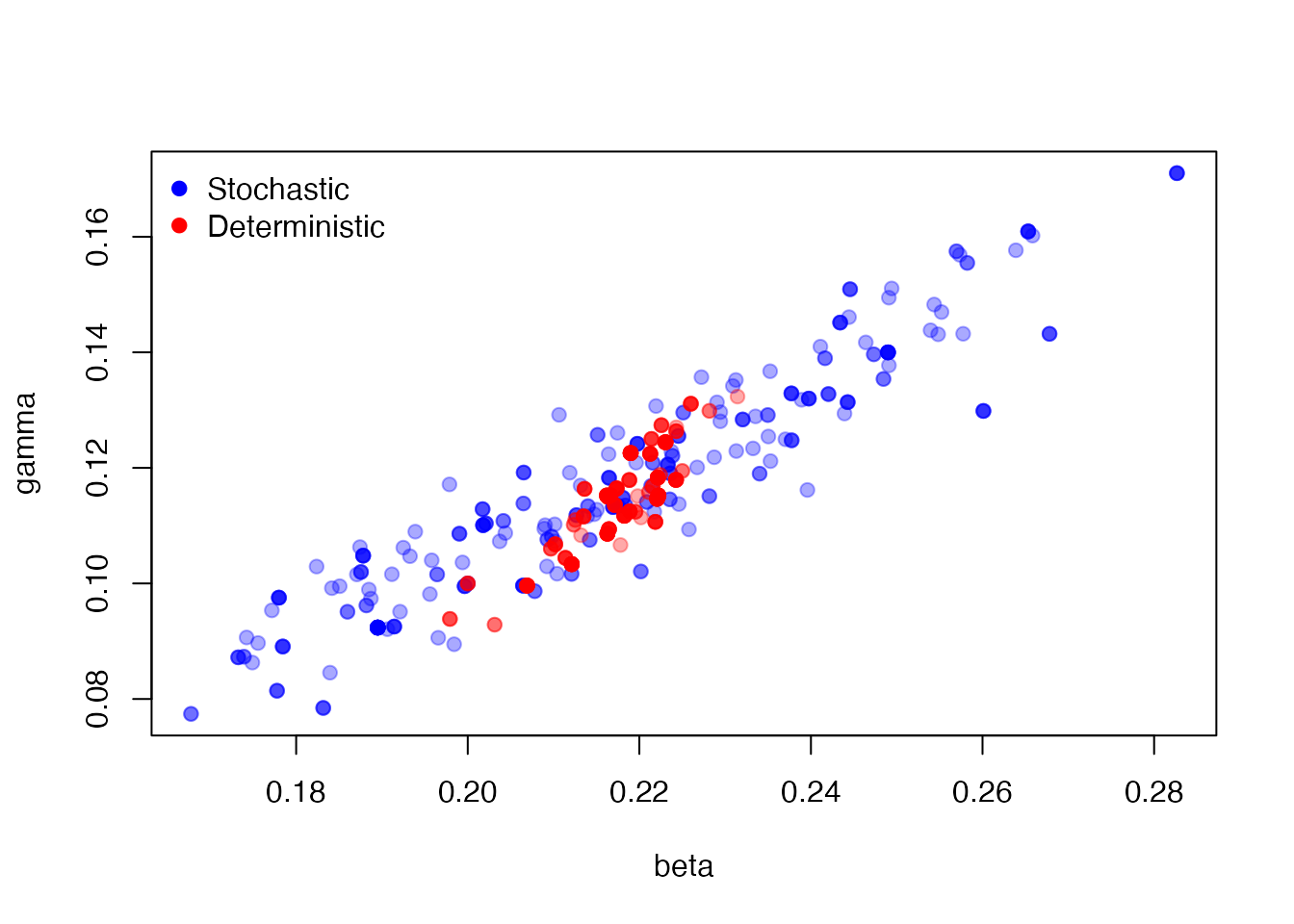
res2 <- mcstate::pmcmc(pars, p2, control = control)

Here, we plot the estimated points for the stochastic (blue) and deterministic (red) parameter samples, showing overlapping but different distributions:

plot(res1$pars, col = "#0000ff55", pch = 19)
points(res2$pars, col = "#ff000055", pch = 19)
legend("topleft", c("Stochastic", "Deterministic"),
       pch = 19, col = c("blue", "red"), bty = "n")