We can test that the SMC algorithm implemented in mcstate::particle_filter() gives an unbiased estimate of the likelihood by comparing a simple model where the likelihood can be calculated exactly. The volatility model included in the dust package fulfils this criteria:
class volatility {
public:
  using real_type = double;
  using internal_type = dust::no_internal;
  using rng_state_type = dust::random::generator<real_type>;

  struct data_type {
    real_type observed;
  };

  struct shared_type {
    real_type alpha;
    real_type sigma;
    real_type gamma;
    real_type tau;
    real_type x0;
  };

  volatility(const dust::pars_type<volatility>& pars) : shared(pars.shared) {
  }

  size_t size() const {
    return 1;
  }

  std::vector<real_type> initial(size_t time, rng_state_type& rng_state) {
    std::vector<real_type> state(1);
    state[0] = shared->x0;
    return state;
  }

  void update(size_t time, const real_type * state,
              rng_state_type& rng_state, real_type * state_next) {
    const real_type x = state[0];
    state_next[0] = shared->alpha * x +
      shared->sigma * dust::random::normal<real_type>(rng_state, 0, 1);
  }

  real_type compare_data(const real_type * state, const data_type& data,
                         rng_state_type& rng_state) {
    return dust::density::normal(data.observed, shared->gamma * state[0],
                                 shared->tau, true);
  }

private:
  dust::shared_ptr<volatility> shared;
};

// Helper function for accepting values with defaults
inline double with_default(double default_value, cpp11::sexp value) {
  return value == R_NilValue ? default_value : cpp11::as_cpp<double>(value);
}

namespace dust {

template <>
dust::pars_type<volatility> dust_pars<volatility>(cpp11::list pars) {
  using real_type = volatility::real_type;
  real_type x0 = 0;
  real_type alpha = with_default(0.91, pars["alpha"]);
  real_type sigma = with_default(1, pars["sigma"]);
  real_type gamma = with_default(1, pars["gamma"]);
  real_type tau = with_default(1, pars["tau"]);

  volatility::shared_type shared{alpha, sigma, gamma, tau, x0};
  return dust::pars_type<volatility>(shared);
}

template <>
volatility::data_type dust_data<volatility>(cpp11::list data) {
  return volatility::data_type{cpp11::as_cpp<double>(data["observed"])};
}

}
This is a dust model; refer to the documentation there for details. This file can be compiled with dust::dust, but here we use the version bundled with dust
volatility <- dust::dust_example("volatility")We can simulate some data from the model:
head(data)
#>   t      value
#> 1 1 -0.6369558
#> 2 2 -0.2570459
#> 3 3 -0.9272309
#> 4 4  1.1763860
#> 5 5  0.8249007
#> 6 6  1.0334913
plot(value ~ t, data, type = "o", pch = 19, las = 1)
In order to estimate the parameters of the process that might have generated this dataset, we need, in addition to our model, an observation/comparison function. In this case, given that we observe some state:
volatility_compare <- function(state, observed, pars) {
  dnorm(observed$value, pars$gamma * drop(state), pars$tau, log = TRUE)
}
We also model the initialisation process:
volatility_initial <- function(info, n_particles, pars) {
  matrix(rnorm(n_particles, 0, pars$sd), 1)
}

pars <- list(
  # Generation process
  alpha = 0.91,
  sigma = 1,
  # Observation process
  gamma = 1,
  tau = 1,
  # Initial condition
  sd = 1)
and preprocess the data into the correct format:
volatility_data <- mcstate::particle_filter_data(data, "t", 1)
#> Warning in mcstate::particle_filter_data(data, "t", 1): 'initial_time' should
#> be provided. I'm assuming '0' which is one time unit before the first time in
#> your data (1), but this might not be appropriate. This will become an error in
#> a future version of mcstate
head(volatility_data)
#>   t_start t_end time_start time_end      value
#> 1       0     1          0        1 -0.6369558
#> 2       1     2          1        2 -0.2570459
#> 3       2     3          2        3 -0.9272309
#> 4       3     4          3        4  1.1763860
#> 5       4     5          4        5  0.8249007
#> 6       5     6          5        6  1.0334913
The particle filter can run with more or fewer particles - this will trade-off runtime with the variance in the estimate, though in a fairly non-linear manner:
n_particles <- 1000With all these pieces we can create our particle filter object with 1000 particles
filter <- mcstate::particle_filter$new(volatility_data, volatility, n_particles,
                                       compare = volatility_compare,
                                       initial = volatility_initial)
filter
#> <particle_filter>
#>   Public:
#>     has_multiple_data: FALSE
#>     has_multiple_parameters: FALSE
#>     history: function (index_particle = NULL)
#>     initialize: function (data, model, n_particles, compare, index = NULL, initial = NULL,
#>     inputs: function ()
#>     model: dust_generator, R6ClassGenerator
#>     n_data: 1
#>     n_parameters: 1
#>     n_particles: 1000
#>     ode_statistics: function ()
#>     restart_state: function (index_particle = NULL, save_restart = NULL, restart_match = FALSE)
#>     run: function (pars = list(), save_history = FALSE, save_restart = NULL,
#>     run_begin: function (pars = list(), save_history = FALSE, save_restart = NULL,
#>     set_n_threads: function (n_threads)
#>     state: function (index_state = NULL)
#>   Private:
#>     compare: function (state, observed, pars)
#>     constant_log_likelihood: NULL
#>     data: particle_filter_data_single, particle_filter_data_discrete, particle_filter_data, data.frame
#>     data_split: list
#>     gpu_config: NULL
#>     index: NULL
#>     initial: function (info, n_particles, pars)
#>     last_history: NULL
#>     last_model: NULL
#>     last_restart_state: NULL
#>     last_stages: NULL
#>     last_state: NULL
#>     n_threads: 1
#>     ode_control: NULL
#>     seed: NULL
#>     stochastic_schedule: NULL
#>     times: 0 1 2 3 4 5 6 7 8 9 10 11 12 13 14 15 16 17 18 19 20 21  ...
Running the particle filter simulates the process on all \(10^3\) particles and compares at each timestep the simulated data with your observed data using the provided comparison function. It returns the log-likelihood:
filter$run(pars)
#> [1] -198.0669
This is stochastic and each time you run it, the estimate will differ:
filter$run(pars)
#> [1] -197.6714
In this case the model is simple enough that we can use a Kalman Filter to calculate the likelihood exactly:
kalman_filter <- function(alpha, sigma, gamma, tau, data) {
  y <- data$value

  mu <- 0
  s <- 1
  log_likelihood <- 0

  for (t in seq_along(y)) {
    mu <- alpha * mu
    s <- alpha^2 * s + sigma^2
    m <- gamma * mu

    S <- gamma^2 * s + tau^2
    K <- gamma * s / S

    mu <- mu + K * (y[t] - m)
    s <- s - gamma * K * s

    log_likelihood <- log_likelihood + dnorm(y[t], m, sqrt(S), log = TRUE)
  }

  log_likelihood
}
ll_k <- kalman_filter(pars$alpha, pars$sigma, pars$gamma, pars$tau,
                      volatility_data)
ll_k
#> [1] -197.4294
Unlike the particle filter the Kalman filter is deterministic:
kalman_filter(pars$alpha, pars$sigma, pars$gamma, pars$tau, volatility_data)
#> [1] -197.4294
However, the particle filter, run multiple times, will create a distribution centred on this likelihood:
n_replicates <- 200
ll <- replicate(n_replicates, filter$run(pars))
hist(ll, col = "steelblue3")
abline(v = ll_k, col = "red", lty = 2, lwd = 2)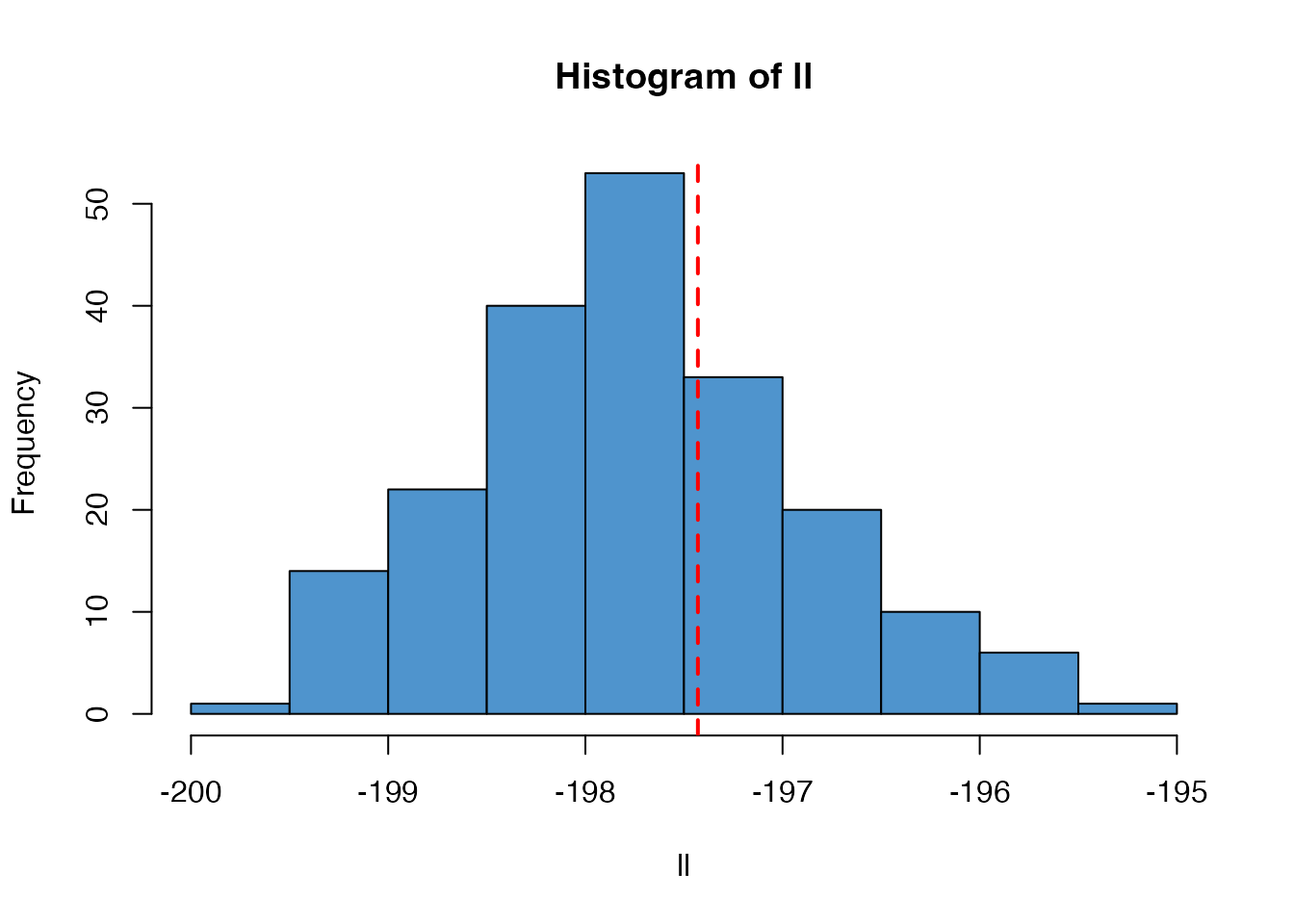
As the number of particles used changes, the variance of this estimate will change
filter2 <- mcstate::particle_filter$new(volatility_data, volatility,
                                        n_particles / 10,
                                        compare = volatility_compare,
                                        initial = volatility_initial)
ll2 <- replicate(n_replicates, filter2$run(pars))
hist(ll2, col = "steelblue3")
abline(v = ll_k, col = "red", lty = 2, lwd = 2)
abline(v = range(ll), col = "orange", lty = 3, lwd = 2)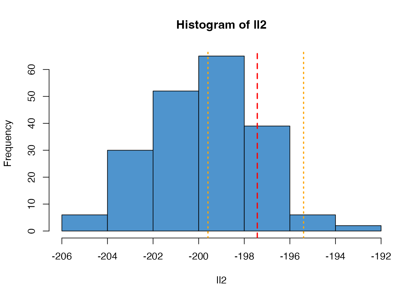
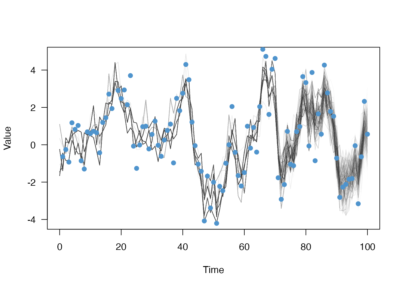
If you run a particle filter with save_history = TRUE, it will record the (filtered) trajectories:s
filter$run(pars, save_history = TRUE)
#> [1] -195.6484
dim(filter$history())
#> [1]    1 1000  101
This is a N state (here 1) x N particles (1000) x N time steps (100) 3d array, but we will drop the first rank of this for plotting
matplot(0:100, t(drop(filter$history())), xlab = "Time", ylab = "Value",
        las = 1, type = "l", lty = 1, col = "#00000002")
points(value ~ t, data, col = "steelblue3", pch = 19)