Vector Control: Indoor Residual Spraying

# Load the requisite packages:
library(malariasimulation)
library(malariaEquilibrium)
# Set colour palette:
cols <- c("#E69F00", "#56B4E9", "#009E73", "#F0E442", "#0072B2", "#D55E00", "#CC79A7")

Indoor Residual Spraying (IRS) involves periodically treating indoor walls with insecticides to eliminate adult female mosquitoes that rest indoors. malariasimulation can be used to investigate the effect of malaria control strategies that deploy IRS. Users can set IRS in the model using the set_spraying() function to parameterise the time and coverage of spraying campaigns.

We will create a few plotting functions to visualise the output.

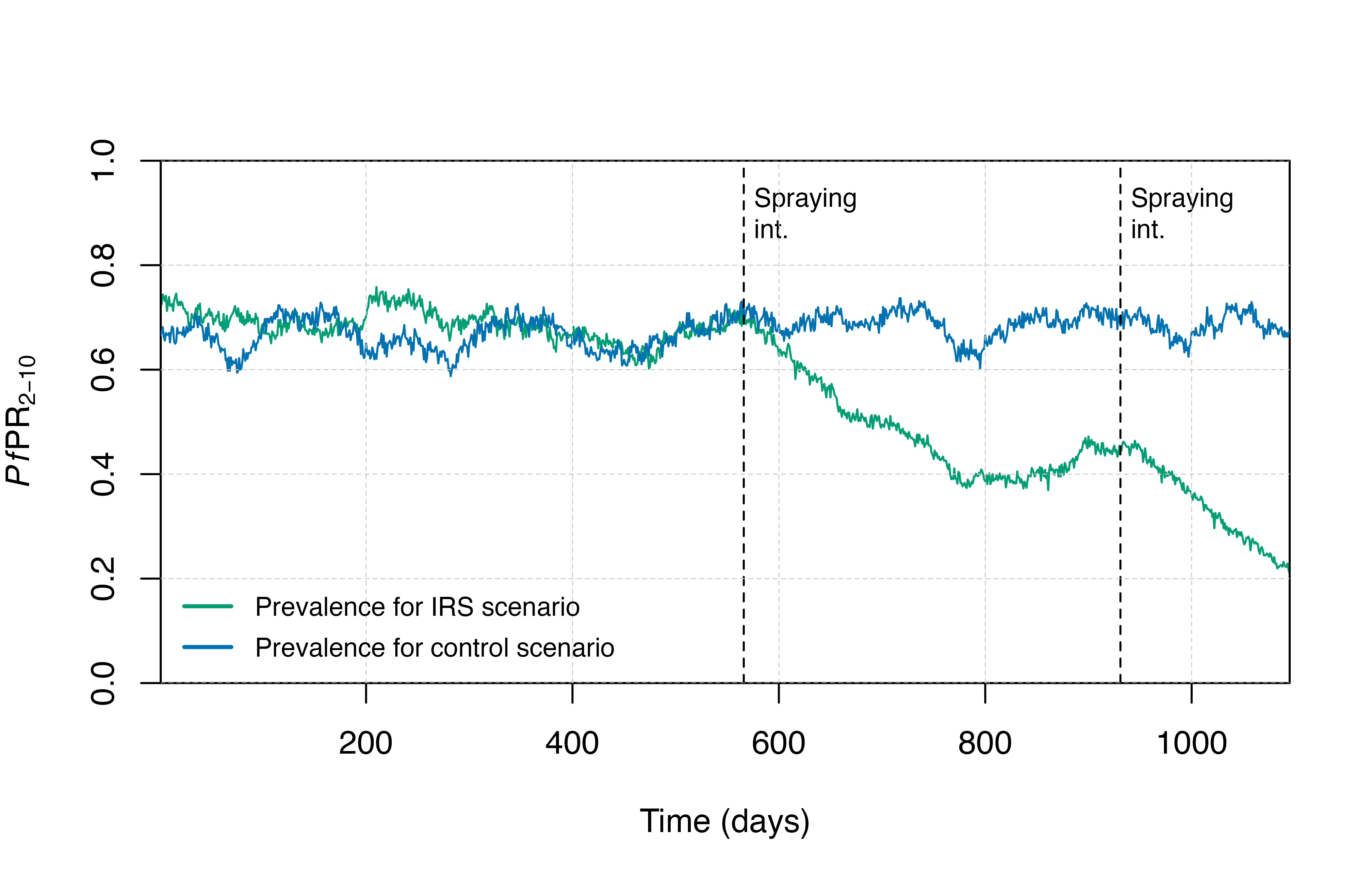
# Plotting functions
plot_prev <- function() {
  plot(x = output$timestep, y = output$n_detect_730_3650 / output$n_730_3650, 
       type = "l", col = cols[3], lwd = 1,
       xlab = "Time (days)", ylab = expression(paste(italic(Pf),"PR"[2-10])),
       xaxs = "i", yaxs = "i", ylim = c(0,1))
  lines(x = output_control$timestep, y = output_control$n_detect_730_3650 / output_control$n_730_3650,
        col = cols[5], lwd = 1)
  abline(v = sprayingtimesteps, lty = 2, lwd = 1, col = "black")
  text(x = sprayingtimesteps + 10, y = 0.9, labels = "Spraying\nint.", adj = 0, cex = 0.8)
  grid(lty = 2, col = "grey80", lwd = 0.5)
  legend("bottomleft", box.lty = 0, 
         legend = c("Prevalence for IRS scenario","Prevalence for control scenario"),
         col = c(cols[3], cols[5]), lty = c(1,1), lwd = 2, cex = 0.8, y.intersp = 1.3)
}

Setting IRS parameters

Parameterisation

Use the get_parameters() function to generate a list of parameters, accepting most of the default values, but modifying seasonality values to model a seasonal setting. Then, we use the set_equilibrium() function to to initialise the model at a given entomological innoculation rate (EIR).

year <- 365
month <- 30
sim_length <- 3 * year
human_population <- 1000
starting_EIR <- 50

simparams <- get_parameters(
  list(
    human_population = human_population,
    # seasonality parameters
    model_seasonality = TRUE, 
    g0 = 0.285277,
    g = c(-0.0248801, -0.0529426, -0.0168910),
    h = c(-0.0216681, -0.0242904, -0.0073646)
  )
)

simparams <- set_equilibrium(parameters = simparams, init_EIR = starting_EIR)

# Running simulation with no IRS
output_control <- run_simulation(timesteps = sim_length, parameters = simparams)

A note on mosquito species

It is also possible to use the set_species() function to account for 3 different mosquito species in the simulation. In this case, the matrices would need to have additional column corresponding to each mosquito species. For example, if we specified that there were 3 species of mosquitoes in the model and nets were distributed at two timesteps, then the matrices would have 2 rows and 3 columns. If you are not already familiar with the set_species() function, see the Mosquito Species vignette.

The default parameters are set to model Anopheles gambiae.

simparams$species
#> [1] "gamb"
simparams$species_proportions
#> [1] 1

Simulation

Then we can run the simulations for a variety of IRS strategies. In the example below, there are two rounds of IRS, the first at 30% coverage and the second at 80% coverage, each 3 months prior to peak rainfall for that year. The function peak_season_offset() outputs a timestep when peak rainfall will be observed based on the seasonality profile we set above. Notice that the matrices specified for the parameters for ls_theta, ls_gamma, ks_theta, ks_gamma, ms_theta, and ms_gamma have two rows, one for each timestep where IRS is implemented, and a number of columns corresponding to mosquito species. In this example, we only have 1 column because the species is set to “gamb” as we saw above.

The structure for the IRS model is documented in the supplementary information from Table 3 in the Supplementary Information of Sherrard-Smith et al., 2018. Table S2.1 in the Supplementary Appendix of Sherrard-Smith et al., 2022 has parameter estimates for insecticide resistance for IRS.

peak <- peak_season_offset(simparams)

sprayingtimesteps <- c(1, 2) * year + peak - 3 * month # A round of IRS is implemented in the 1st and second year 3 months prior to peak transmission.

sprayingparams <- set_spraying(
  simparams,
  timesteps = sprayingtimesteps,
  coverages = c(0.3, 0.8), # # The first round covers 30% of the population and the second covers 80%. 
  ls_theta = matrix(2.025, nrow=length(sprayingtimesteps), ncol=1), # Matrix of mortality parameters; nrows=length(timesteps), ncols=length(species) 
  ls_gamma = matrix(-0.009, nrow=length(sprayingtimesteps), ncol=1), # Matrix of mortality parameters per round of IRS and per species
  ks_theta = matrix(-2.222, nrow=length(sprayingtimesteps), ncol=1), # Matrix of feeding success parameters per round of IRS and per species
  ks_gamma = matrix(0.008, nrow=length(sprayingtimesteps), ncol=1), # Matrix of feeding success parameters per round of IRS and per species
  ms_theta = matrix(-1.232, nrow=length(sprayingtimesteps), ncol=1), # Matrix of deterrence parameters per round of IRS and per species
  ms_gamma = matrix(-0.009, nrow=length(sprayingtimesteps), ncol=1) # Matrix of deterrence parameters per round of IRS and per species
)

output <- run_simulation(timesteps = sim_length, parameters = sprayingparams)

Visualisation

# Plot prevalence
plot_prev()