Stochastic Variation • malariasimulation

# Load the requisite packages:
library(malariasimulation)
# Set colour palette:
cols <- c("#E69F00", "#56B4E9", "#009E73", "#F0E442", "#0072B2", "#D55E00", "#CC79A7")
set.seed(555)
knitr::opts_chunk$set(
  collapse = TRUE,
  comment = "#>",
  dpi=300,
  fig.width=7
)

malariasimulation is a stochastic, individual-based model and, as such, simulations run with identical parameterisations will generate non-identical, sometimes highly variable, outputs. To illustrate this, we will compare the prevalence and incidence of malaria over a year in simulations with a small and a larger population. Then we will demonstrate how this variation can be estimated by running multiple simulations using the run_simulation_with_repetitions function.

First, we will create a few plotting functions to visualise outputs.

plot_prev <- function(output, ylab = TRUE, ylim = c(0,1)){
  if (ylab == TRUE) {
    ylab = "Prevalence in children aged 2-10 years"
    } else {ylab = ""}
  plot(x = output$timestep, y = output$n_detect_730_3650 / output$n_730_3650, 
       type = "l", col = cols[3], ylim = ylim,
       xlab = "Time (days)", ylab = ylab, lwd = 1,
       xaxs = "i", yaxs = "i")
  grid(lty = 2, col = "grey80", lwd = 0.5)
}

plot_inci <- function(output, ylab = TRUE, ylim){
  if (ylab == TRUE) {
    ylab = "Incidence per 1000 children aged 0-5 years"
    } else {ylab = ""}
  plot(x = output$timestep, y = output$n_inc_clinical_0_1825 / output$n_0_1825 * 1000, 
       type = "l", col = cols[5], ylim = ylim,
       xlab = "Time (days)", ylab = ylab, lwd = 1,
       xaxs = "i", yaxs = "i")
  grid(lty = 2, col = "grey80", lwd = 0.5)
}

aggregate_function <- function(df){
  tmp <- aggregate(
    df$n_detect_730_3650,
    by=list(df$timestep),
    FUN = function(x) {
      c(median = median(x),
        lowq = unname(quantile(x, probs = .25)),
        highq = unname(quantile(x, probs = .75)),
        mean = mean(x),
        lowci = mean(x) - 1.96*sd(x),
        highci = mean(x) + 1.96*sd(x)
      )
      }
  )
  data.frame(cbind(t = tmp$Group.1, tmp$x))
}

plot_variation_function <- function(df, title_str){
  plot(type="n", xlim=c(0,max(df$t)),
       c(1,1),
       ylim = c(-4, 14),
       xaxs = "i", yaxs = "i",
       xlab = 'timestep', ylab ='Light miscroscopy detectable infections', main = title_str,
       font.main = 1)
  grid(lty = 2, col = "grey80", lwd = 0.5)
  polygon(x = c(df$t,rev(df$t)), y = c(df$highci, rev(df$lowci)), col = cols[2], border = cols[2])
  polygon(x = c(df$t,rev(df$t)), y = c(df$highq, rev(df$lowq)), col = cols[5], border = cols[5])
  points(x = df$t, y = df$median, type = "l", ylim = c(25,40), lwd = 2, col = "black")
}

Variation and population size

Parameterisation

We will use the get_parameters() function to generate a list of parameters, accepting the default values, for two different population sizes and use the set_equilibrium() function to initialise the model at a given entomological inoculation rate (EIR). The only parameter which changes between the two parameter sets is the argument for human_population.

# A small population 
simparams_small <- get_parameters(list(
  human_population = 1000,
  clinical_incidence_rendering_min_ages = 0,
  clinical_incidence_rendering_max_ages = 5 * 365,
  individual_mosquitoes = FALSE
))

simparams_small <- set_equilibrium(parameters = simparams_small, init_EIR = 50)

# A larger population 
simparams_big <- get_parameters(list(
  human_population = 10000,
  clinical_incidence_rendering_min_ages = 0,
  clinical_incidence_rendering_max_ages = 5 * 365,
  individual_mosquitoes = FALSE
))

simparams_big <- set_equilibrium(parameters = simparams_big, init_EIR = 50)

Simulations

The n_detect_730_3650 output below shows the total number of individuals in the age group rendered (here, 730-3650 timesteps or 2-10 years) who have microscopy-detectable malaria. Notice that the output is smoother at a higher population.

Some outcomes will be more sensitive than others to stochastic variation even with the same population size. In the plots below, prevalence is smoother than incidence even at the same population. This is because prevalence is a measure of existing infection, while incidence is recording new cases per timestep.

# A small population
output_small_pop <- run_simulation(timesteps = 365, parameters = simparams_small)

# A larger population
output_big_pop <- run_simulation(timesteps = 365, parameters = simparams_big)

# Plotting 
par(mfrow = c(2,2))
plot_prev(output_small_pop, ylim = c(0.5, 0.8)); title(expression(paste(italic(Pf),"PR"[2-10], " at n = 1,000")))
plot_inci(output_small_pop, ylim = c(0, 25)); title("Incidence per 1000 children at n = 1,000", cex.main = 1, font.main = 1)
plot_prev(output_big_pop, ylim = c(0.5, 0.8)); title(expression(paste(italic(Pf),"PR"[2-10], " at n = 10,000")))
plot_inci(output_big_pop, ylim = c(0, 25)); title("Incidence per 1000 children at n = 10,000", cex.main = 1, font.main = 1)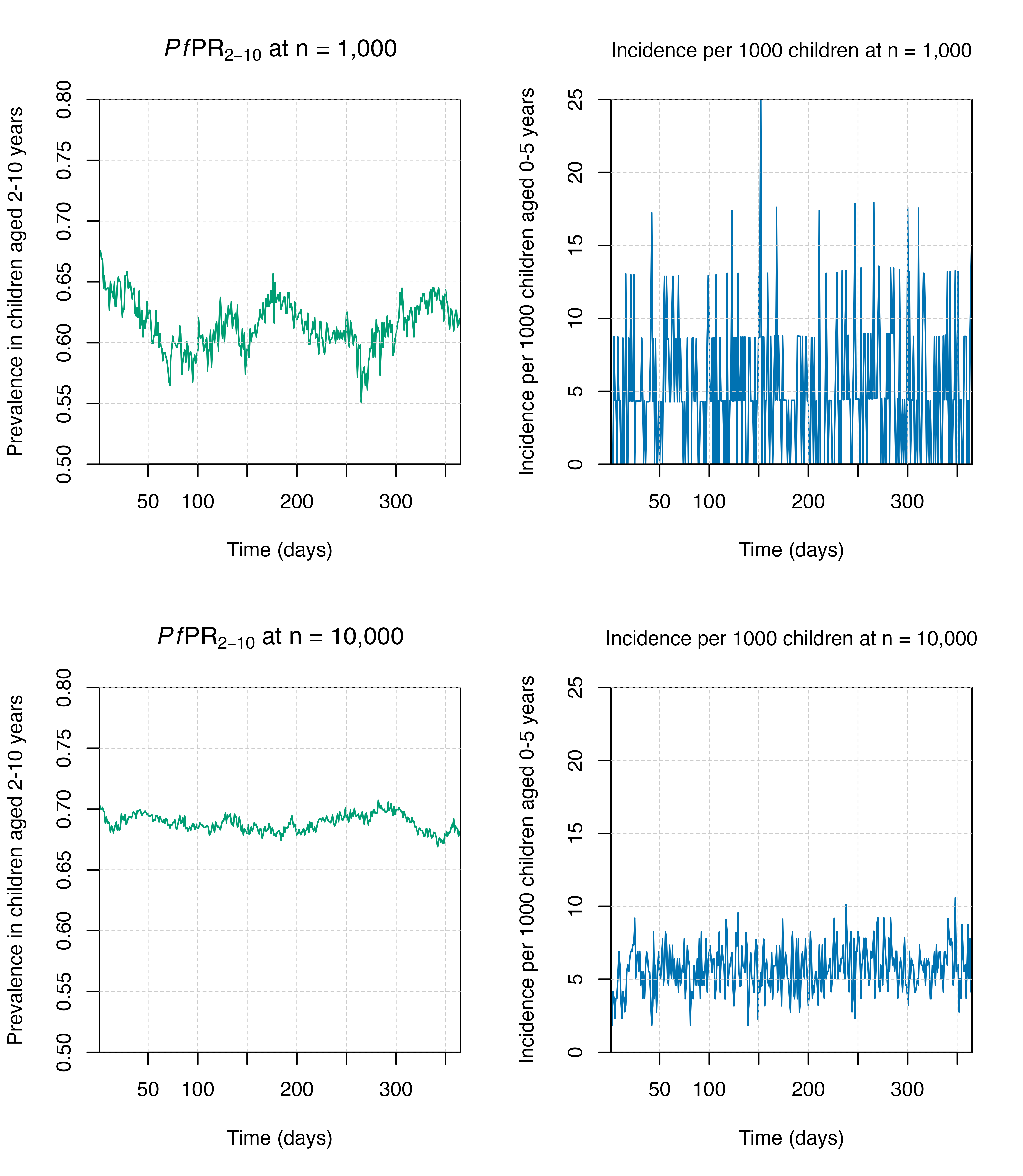

Stochastic elimination

With stochastic models, random elimination of malaria in a small population with low transmisison may happen. In the example below, we run two simulations: one with a very small population, and one with a larger population. There is stochastic fade out (elimination) in the smaller population, while the larger population has stable transmission over time. For this reason, it is important to run models with large-enough populations to avoid stochastic elimination.

# A small population 
simparams_small <- get_parameters(list(
  human_population = 50,
  clinical_incidence_rendering_min_ages = 0,
  clinical_incidence_rendering_max_ages = 5 * 365,
  individual_mosquitoes = FALSE
))

simparams_small <- set_equilibrium(parameters = simparams_small, init_EIR = 1)

# A larger population 
simparams_big <- get_parameters(list(
  human_population = 1000,
  clinical_incidence_rendering_min_ages = 0,
  clinical_incidence_rendering_max_ages = 5 * 365,
  individual_mosquitoes = FALSE
))

simparams_big <- set_equilibrium(parameters = simparams_big, init_EIR = 1)

Simulations

set.seed(444)
# A small population
output_small_pop <- run_simulation(timesteps = 365 * 2, parameters = simparams_small)

# A larger population
output_big_pop <- run_simulation(timesteps = 365 * 2, parameters = simparams_big)

# Plotting 
par(mfrow = c(1, 2))
plot_prev(output_small_pop, ylim = c(0, 0.2)); title(expression(paste(italic(Pf),"PR"[2-10], " at n = 50")))
plot_prev(output_big_pop, ylab = FALSE, ylim = c(0, 0.2)); title(expression(paste(italic(Pf),"PR"[2-10], " at n = 1,000")))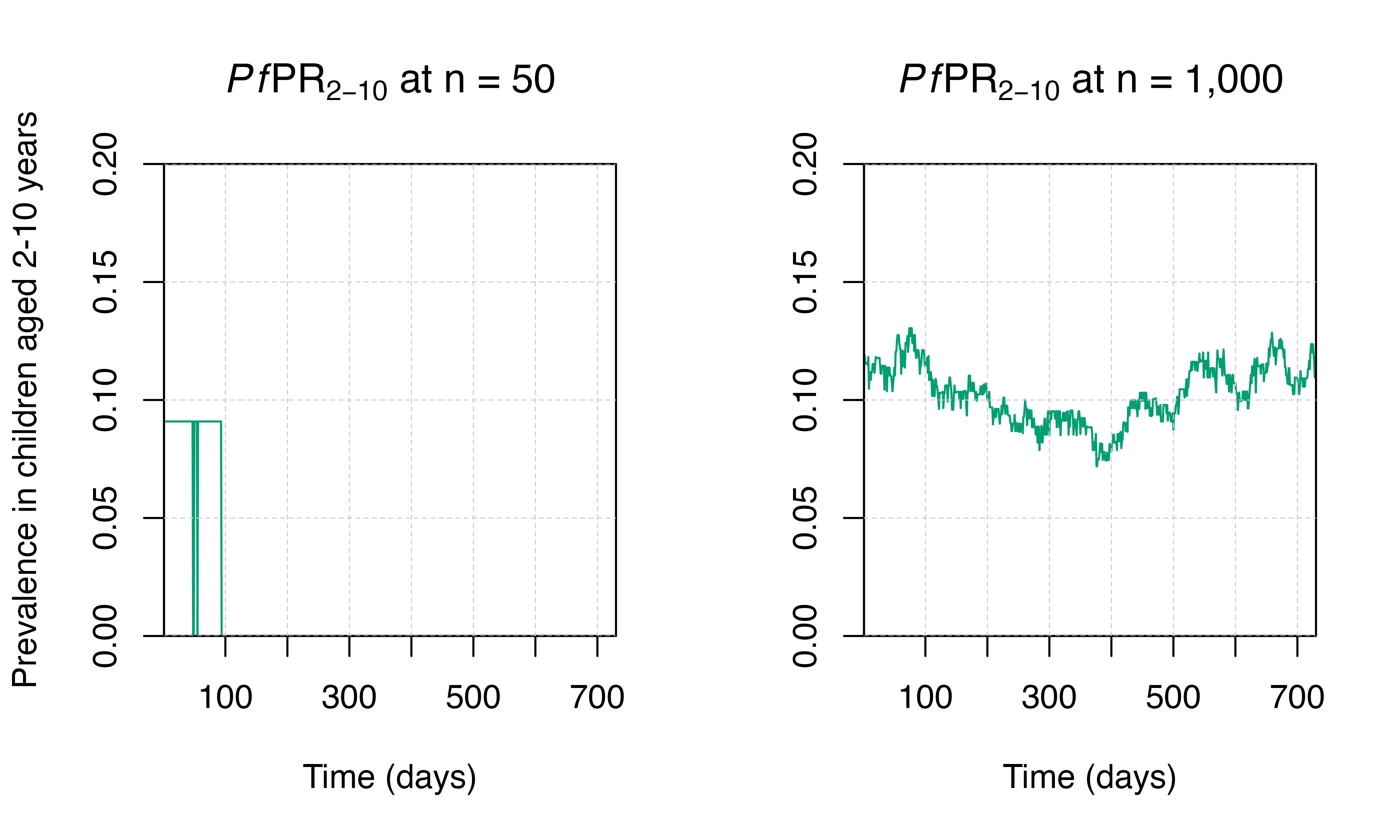

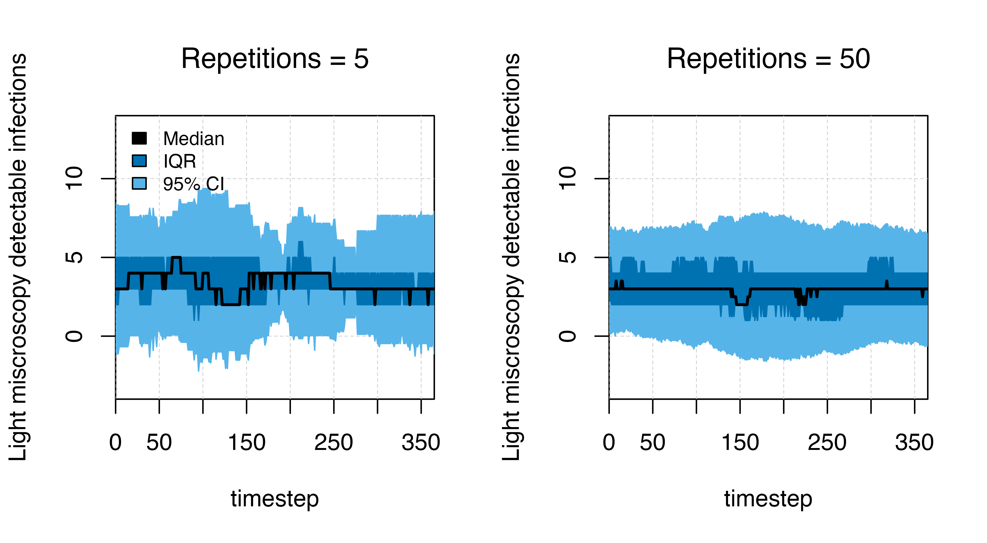
Estimating variation

We can estimate the variation in the number of detectable cases by repeating the simulation several times using the run_simulation_with_repetitions() function. The functions requires arguments for repetitions (the number of repeat simulations) and the option of whether to run simulations in parallel (where available: parallel = T), in addition to the standard timesteps and parameter list.

simparams <- get_parameters() |>  set_equilibrium(init_EIR = 1)

output_few_reps <- run_simulation_with_repetitions(
  timesteps = 365,
  repetitions = 5,
  overrides = simparams,
  parallel=TRUE
)

output_many_reps <- run_simulation_with_repetitions(
  timesteps = 365,
  repetitions = 50,
  overrides = simparams,
  parallel=TRUE
)

# Aggregate the data
df_few <- aggregate_function(output_few_reps)
df_many <- aggregate_function(output_many_reps)

par(mfrow = c(1,2))
plot_variation_function(df = df_few, title_str = "Repetitions = 5")
legend("topleft", legend = c("Median", "IQR", "95% CI"), ncol = 1, 
       fill = c("black", cols[5], cols[2]), cex = 0.8, bty = "n")
plot_variation_function(df = df_many, title_str = "Repetitions = 50")