Double well

Bob Verity and Pete Winskill

2021-12-16

Purpose: to compare drjacoby results for a challenging problem involving a multimodal posterior, both with and without temperature rungs.

Model

We assume a single parameter mu drawn from a double well potential distribution, defined by the formula:

\[ \begin{aligned} \mu &\propto exp\left(-\gamma(\mu^2 - 1)^2\right) \end{aligned} \] where \(\gamma\) is a parameter that defines the strength of the well (higher \(\gamma\) leads to a deeper valley and hence more challenging problem). NB, there is no data in this example, as the likelihood is defined exactly by these parameters.

Likelihood and prior:

Parameters dataframe:

L <- 2
gamma <- 30
df_params <- define_params(name = "mu", min = -L, max = L,
                           name = "gamma", min = gamma, max = gamma)

Single temperature rung (no Metropolis coupling)

mcmc <- run_mcmc(data = list(x = -1),
                 df_params = df_params,
                 loglike = "loglike",
                 logprior = "logprior",
                 burnin = 1e3,
                 samples = 1e5,
                 chains = 1,
                 rungs = 1,
                 silent = TRUE)

# trace plot
plot_par(mcmc, show = "mu")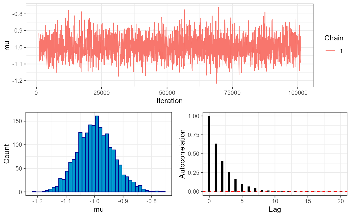

# extract posterior draws
output_sub <- subset(mcmc$output, phase == "sampling")
mu_draws <- output_sub$mu

# get analytical solution
x <- seq(-L, L, l = 1001)
fx <- exp(-gamma*(x^2 - 1)^2)
fx <- fx / sum(fx) * 1/(x[2]-x[1])

# overlay plots
hist(mu_draws, breaks = seq(-L, L, l = 201), probability = TRUE, main = "", col = "black")
lines(x, fx, col = 2, lwd = 2)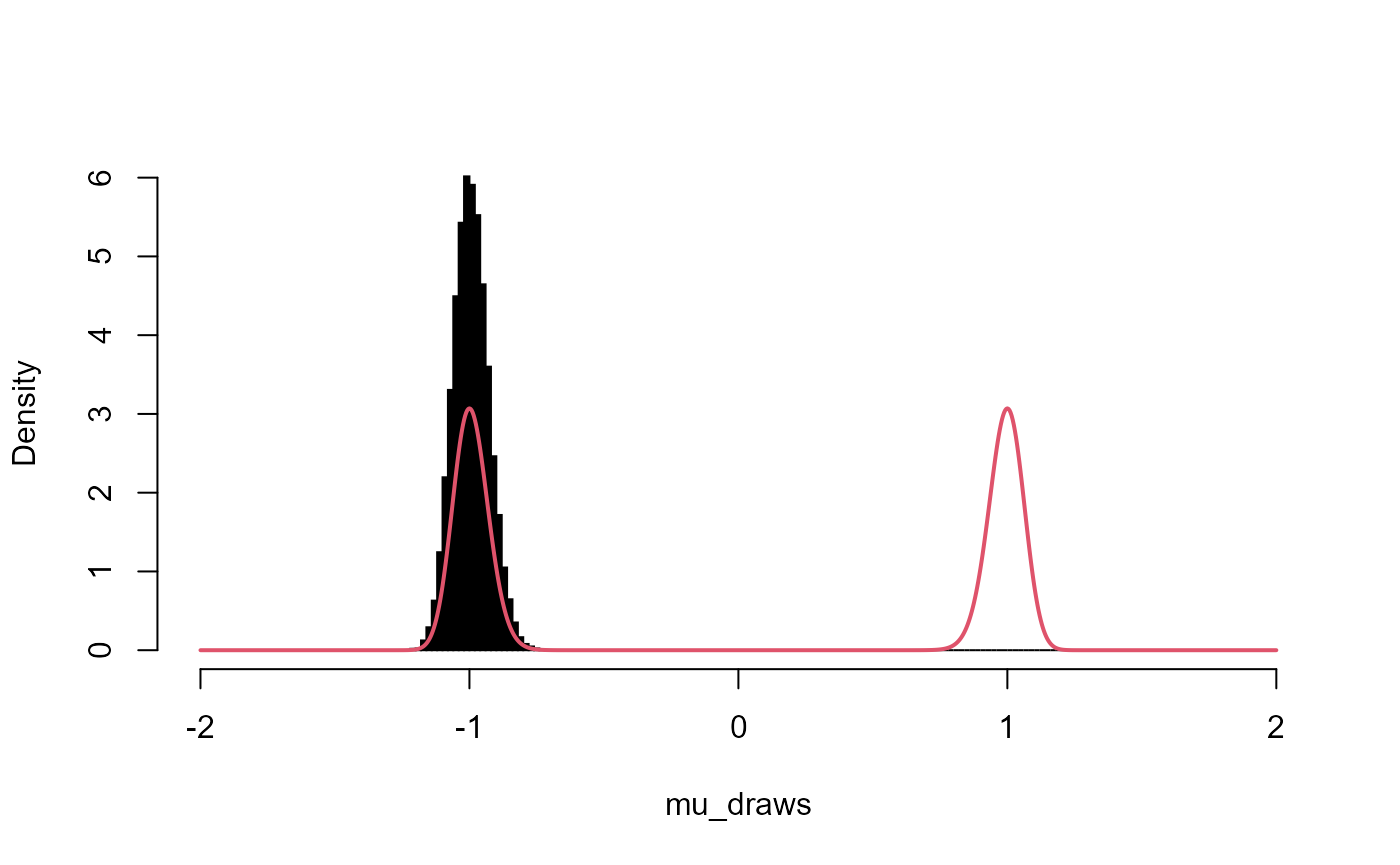

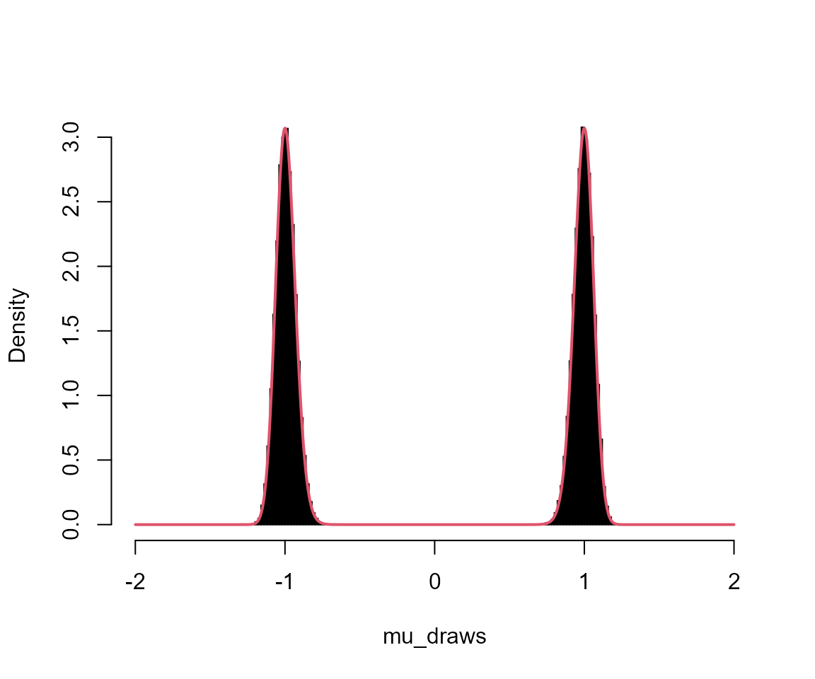
Multiple temperature rungs

mcmc <- run_mcmc(data = list(x = -1),
                 df_params = df_params,
                 loglike = "loglike",
                 logprior = "logprior",
                 burnin = 1e3,
                 samples = 1e5,
                 chains = 1,
                 rungs = 11,
                 alpha = 2,
                 pb_markdown = TRUE)

## MCMC chain 1
## burn-in
## 
  |                                                                            
  |======================================================================| 100%
## acceptance rate: 21.7%
## sampling phase
## 
  |                                                                            
  |======================================================================| 100%
## acceptance rate: 22%
## chain completed in 4.397968 seconds

## total MCMC run-time: 4.4 seconds

# trace plot
plot_par(mcmc, show = "mu")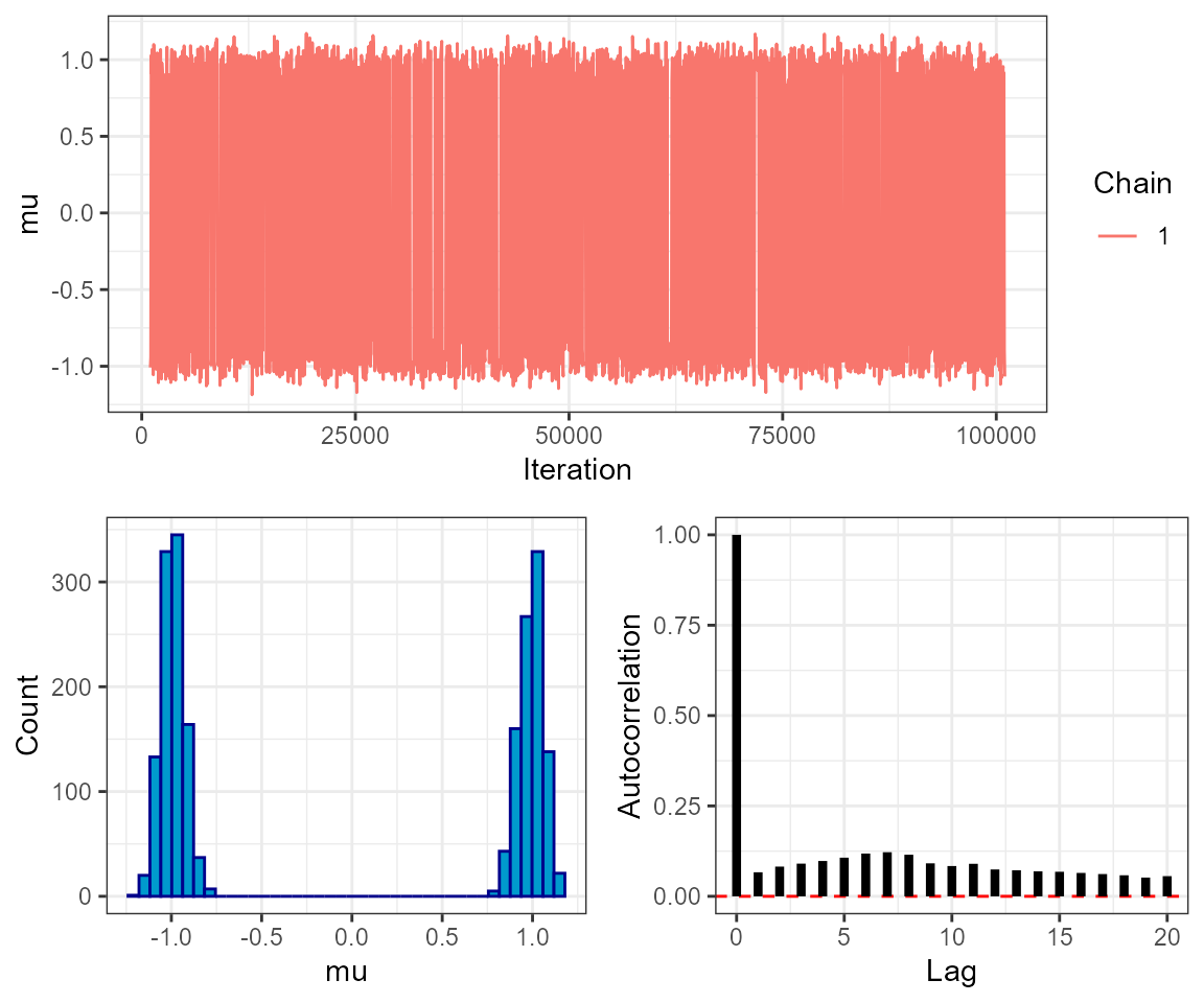

# coupling acceptance plot
plot_mc_acceptance(mcmc)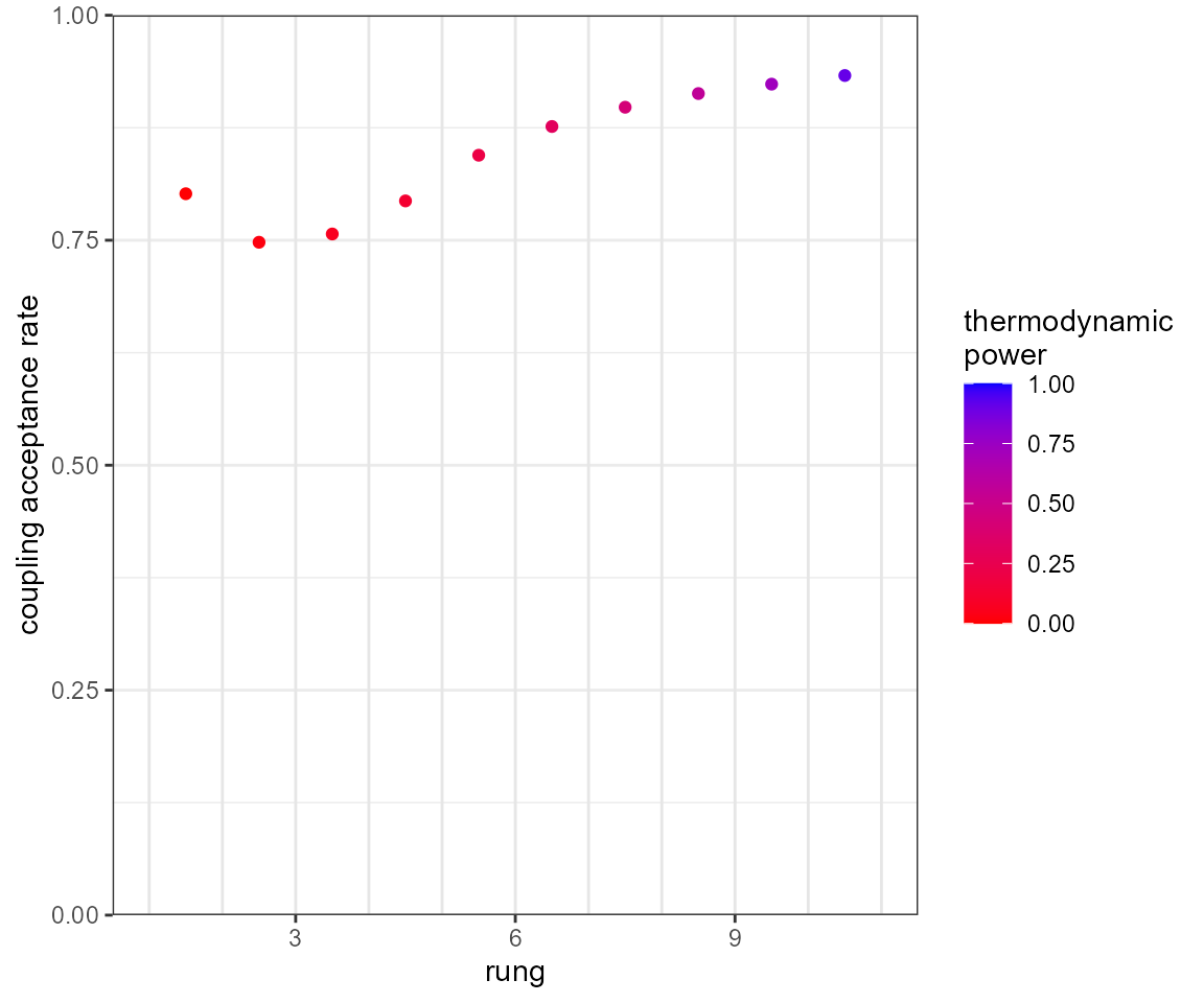

# extract posterior draws
output_sub <- subset(mcmc$output, phase == "sampling")
mu_draws <- output_sub$mu

# overlay plots
hist(mu_draws, breaks = seq(-L, L, l = 201), probability = TRUE, main = "", col = "black")
lines(x, fx, col = 2, lwd = 2)