Building a model with odin
odin
- A “domain specific language”
- Originally designed for ordinary differential equations
- Subsequently extended to difference equations (enabling discrete-time stochastic models)
- Refined into second version
odin2
odin
A script containing the code featured in these slides can be downloaded here.
ODE models
\[\begin{gather*} \frac{dS}{dt} = -\beta S \frac{I}{N}\\ \frac{dI}{dt} = \beta S \frac{I}{N} - \gamma I\\ \frac{dR}{dt} = \gamma I \end{gather*}\]
In the book: Getting started with odin
Things to note:
- out of order definition
- every variable has
initialandderivpair - parameters declared with
parameter(), default values can be given in brackets though not required
Compiling the model with odin2
You can also compile code from a file by its path e.g. odin("models/sir-basic.R").
In the book: Getting started with odin
Running the model with dust2
The output has dimensions number of states x number of timepoints
In the book: Getting started with odin
Unpacking states
Output can be nicely unpacked into the different states using dust_unpack_state
In the book: Getting started with odin
Setting the state
Upon creation all systems start with a state full of zeros.
Typically we need to set the state. We used
to set the state according to the initial conditions defined in the odin code. We can also set the state using a new state vector e.g.
In the book: Getting started with odin
Setting the state
The order of states in a system can be found via
or
In the book: Getting started with odin
Inputting parameters (pars)
- We created our system with
pars = list()- an empty list - This means we use all default values for parameters in the odin code
- We can pass in a named list of parameters to use non-default values
- e.g.
pars = list(beta = 0.35, gamma = 0.15)would use those values forbetaandgammaand the default values for all other parameters - You will need to include values for any parameters without default values!
In the book: Getting started with odin
Stochastic models
update(S) <- S - n_SI
update(I) <- I + n_SI - n_IR
update(R) <- R + n_IR

initial(S) <- N - I0
initial(I) <- I0
initial(R) <- 0

p_SI <- 1 - exp(-beta * I / N * dt)
p_IR <- 1 - exp(-gamma * dt)
n_SI <- Binomial(S, p_SI)
n_IR <- Binomial(I, p_IR)

N <- parameter(1000)
I0 <- parameter(10)
beta <- parameter(0.2)
gamma <- parameter(0.1)
\[\begin{gather*} S(t + \Delta t) = S(t) - n_{SI}\\ I(t + \Delta t) = I(t) + n_{SI} - n_{IR}\\ R(t + \Delta t) = R(t) + n_{IR} \end{gather*}\]
dtis a special parameter- every variable has
initialandupdatepair
In the book: Stochasticity
…compared with ODE models
update(S) <- S - n_SI
update(I) <- I + n_SI - n_IR
update(R) <- R + n_IR

initial(S) <- N - I0
initial(I) <- I0
initial(R) <- 0

p_SI <- 1 - exp(-beta * I / N * dt)
p_IR <- 1 - exp(-gamma * dt)
n_SI <- Binomial(S, p_SI)
n_IR <- Binomial(I, p_IR)

N <- parameter(1000)
I0 <- parameter(10)
beta <- parameter(0.2)
gamma <- parameter(0.1)In the book: Stochasticity
Compiling with odin2
sir <- odin({
  update(S) <- S - n_SI
  update(I) <- I + n_SI - n_IR
  update(R) <- R + n_IR

  initial(S) <- N - I0
  initial(I) <- I0
  initial(R) <- 0

  p_SI <- 1 - exp(-beta * I / N * dt)
  p_IR <- 1 - exp(-gamma * dt)
  n_SI <- Binomial(S, p_SI)
  n_IR <- Binomial(I, p_IR)

  N <- parameter(1000)
  I0 <- parameter(10)
  beta <- parameter(0.2)
  gamma <- parameter(0.1)
})
In the book: Stochasticity
Functions in odin2
- we have used the exponential function
exp() - many mathematical functions are supported in
odin2- a full list can be found here
- we have used
Binomial(S, p_SI)for a Binomial random draw withsize = Sandprob = p_SI - many distributions are supported - a full list with their names and parameterisations can be found here
time in odin
timeis a special (continuous) variable inodinmodels- In discrete-time (stochastic) models,
timeis updated in increments of sizedt
In the book: On the nature of time
Running a single simulation
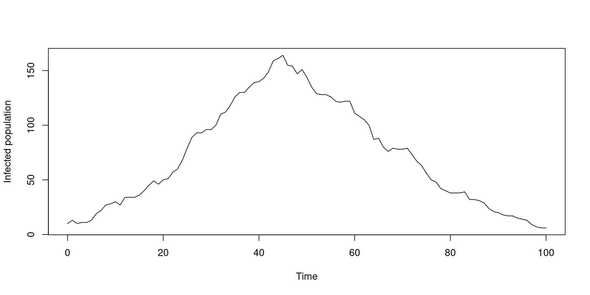
In the book: Stochasticity
Running multiple simulations
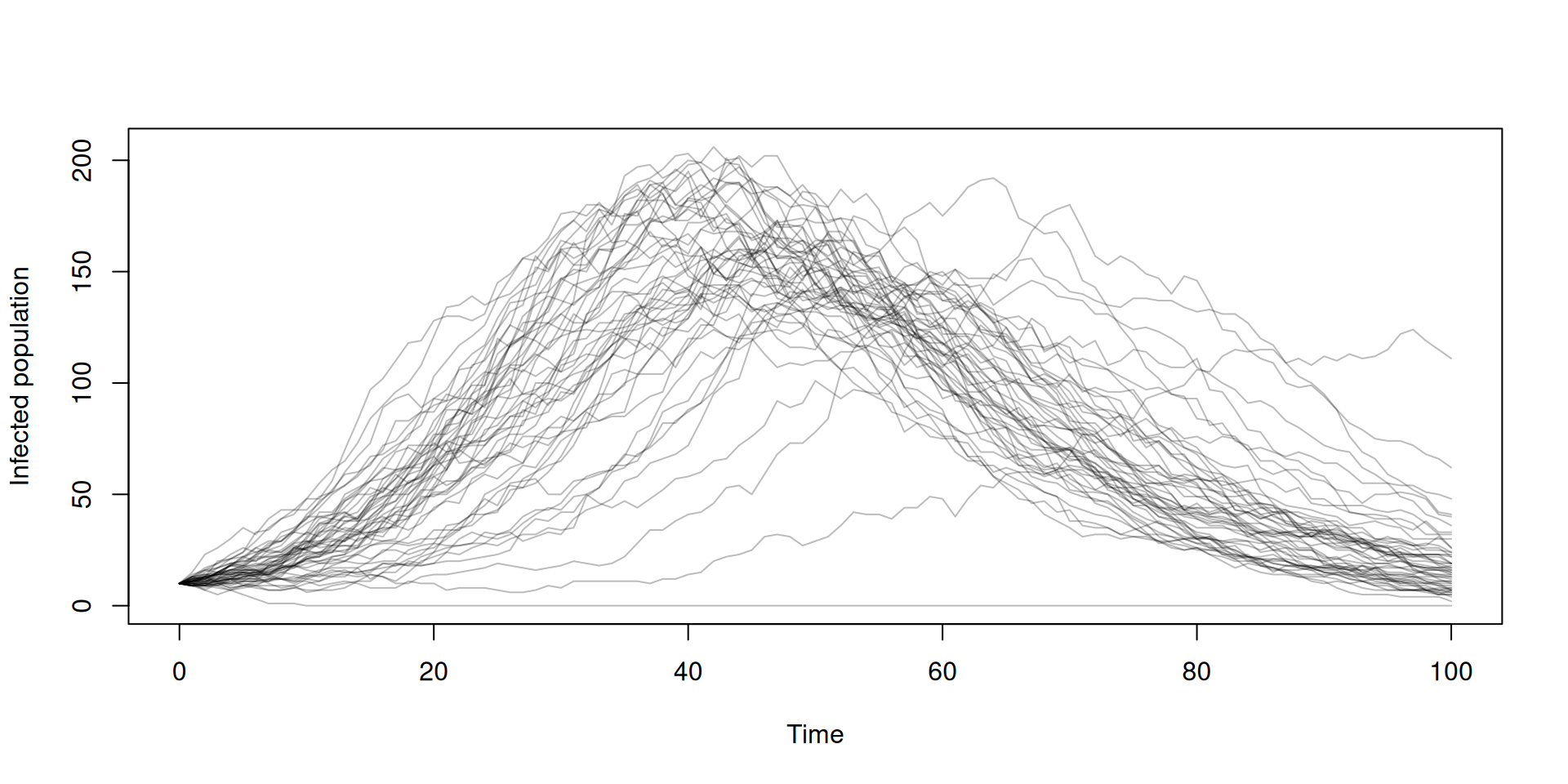
In the book: Stochasticity
Calculating incidence with zero_every
sir <- odin({
  update(S) <- S - n_SI
  update(I) <- I + n_SI - n_IR
  update(R) <- R + n_IR
  update(incidence) <- incidence + n_SI

  p_SI <- 1 - exp(-beta * I / N * dt)
  p_IR <- 1 - exp(-gamma * dt)
  n_SI <- Binomial(S, p_SI)
  n_IR <- Binomial(I, p_IR)

  initial(S) <- N - I0
  initial(I) <- I0
  initial(R) <- 0
  initial(incidence, zero_every = 1) <- 0

  N <- parameter(1000)
  I0 <- parameter(10)
  beta <- parameter(0.2)
  gamma <- parameter(0.1)
})
In the book: On the nature of time
Incidence accumulates then resets
sys <- dust_system_create(sir, pars = list(), dt = 1 / 128)
dust_system_set_state_initial(sys)
t <- seq(0, 20, by = 1 / 128)
y <- dust_system_simulate(sys, t)
y <- dust_unpack_state(sys, y)

plot(t[t %% 1 == 0], y$incidence[t %% 1 == 0], type = "o", pch = 19,
     ylab = "Infection incidence", xlab = "Time")
lines(t, y$incidence, col = "red")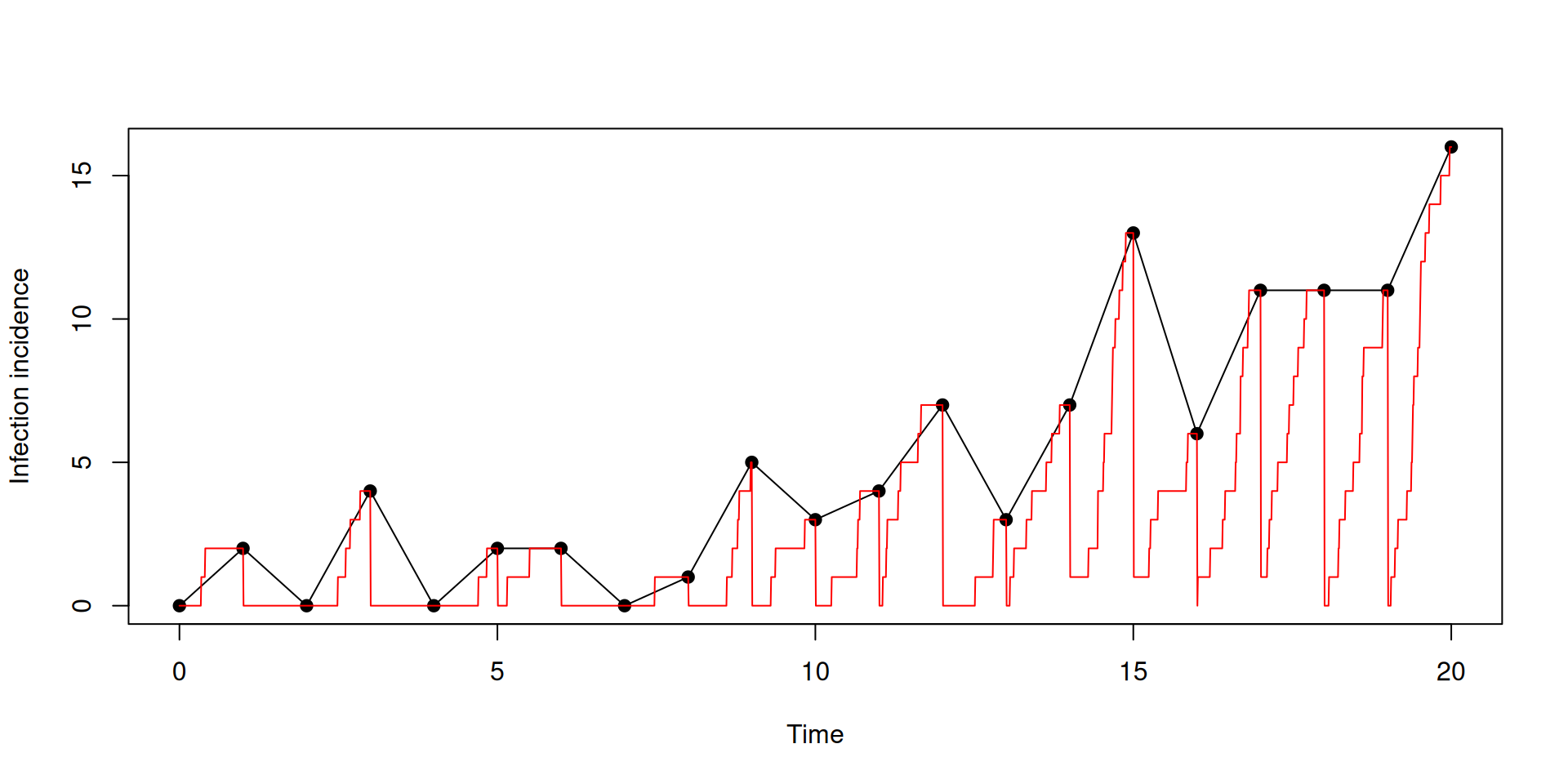
In the book: On the nature of time
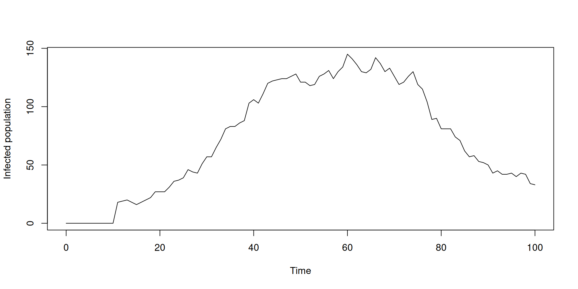
Time-varying inputs: using time
sir <- odin({
  update(S) <- S - n_SI
  update(I) <- I + n_SI - n_IR
  update(R) <- R + n_IR
  update(incidence) <- incidence + n_SI

  seed <- if (time == seed_time) seed_size else 0

  p_SI <- 1 - exp(-beta * I / N * dt)
  p_IR <- 1 - exp(-gamma * dt)
  n_SI <- min(seed + Binomial(S, p_SI), S)
  n_IR <- Binomial(I, p_IR)

  initial(S) <- N
  initial(I) <- 0
  initial(R) <- 0
  initial(incidence, zero_every = 1) <- 0

  N <- parameter(1000)
  beta <- parameter(0.2)
  gamma <- parameter(0.1)
  seed_time <- parameter()
  seed_size <- parameter()
})
In the book: Inputs that vary over time
Time-varying inputs: using time
In the book: Inputs that vary over time
Time-varying inputs: using interpolate
The interpolate function in odin can be used for time-varying parameters, with specification of
- the times of changepoints
- the values at those changepoints
- the type of interpolation: linear, constant or spline
In the book: Inputs that vary over time
Time-varying inputs: using interpolate
sir <- odin({
  update(S) <- S - n_SI
  update(I) <- I + n_SI - n_IR
  update(R) <- R + n_IR
  update(incidence) <- incidence + n_SI

  beta <- interpolate(beta_time, beta_value, "constant")
  beta_time <- parameter()
  beta_value <- parameter()
  dim(beta_time, beta_value) <- parameter(rank = 1)

  p_SI <- 1 - exp(-beta * I / N * dt)
  p_IR <- 1 - exp(-gamma * dt)
  n_SI <- Binomial(S, p_SI)
  n_IR <- Binomial(I, p_IR)

  initial(S) <- N - I0
  initial(I) <- I0
  initial(R) <- 0
  initial(incidence, zero_every = 1) <- 0

  N <- parameter(1000)
  I0 <- parameter(10)
  gamma <- parameter(0.1)
})
In the book: Inputs that vary over time
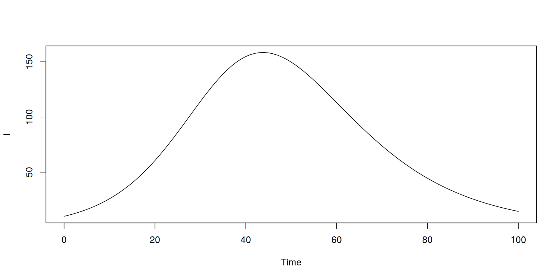
Time-varying inputs: using interpolate
pars <- list(beta_time = c(0, 30), beta_value = c(0.2, 1))
sys <- dust_system_create(sir, pars = pars, dt = 0.25)
dust_system_set_state_initial(sys)
t <- seq(0, 100)
y <- dust_system_simulate(sys, t)
y <- dust_unpack_state(sys, y)

plot(t, y$I, type = "l", xlab = "Time", ylab = "Infected population")
abline(v = 30, lty = 3)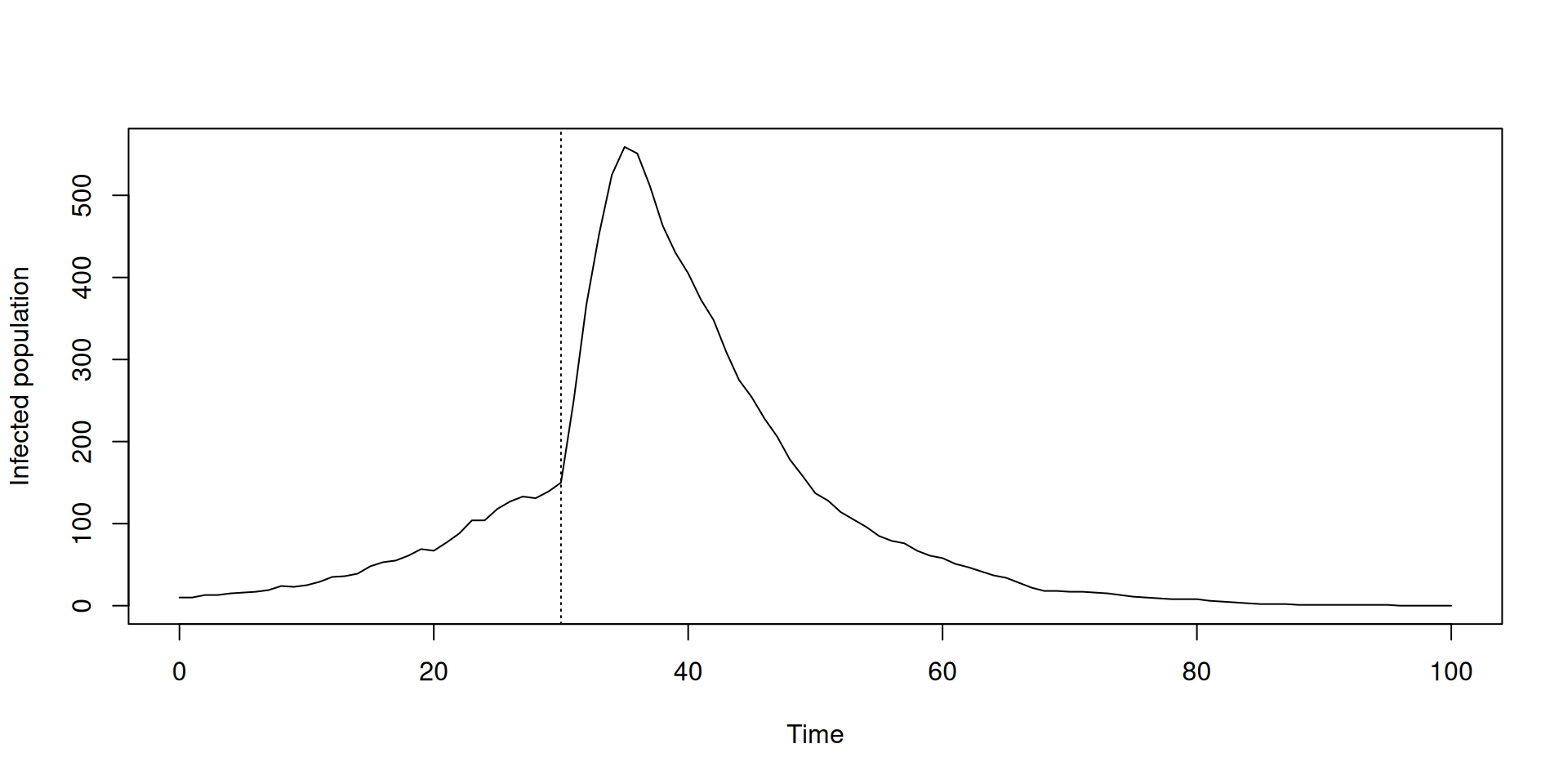
In the book: Inputs that vary over time
Using arrays
sir_age <- odin({
  # Equations for transitions between compartments by age group
  update(S[]) <- S[i] - n_SI[i]
  update(I[]) <- I[i] + n_SI[i] - n_IR[i]
  update(R[]) <- R[i] + n_IR[i]
  update(incidence) <- incidence + sum(n_SI)

  # Individual probabilities of transition:
  p_SI[] <- 1 - exp(-lambda[i] * dt) # S to I
  p_IR <- 1 - exp(-gamma * dt) # I to R

  # Calculate force of infection

  # age-structured contact matrix: m[i, j] is mean number
  # of contacts an individual in group i has with an
  # individual in group j per time unit
  m <- parameter()

  # here s_ij[i, j] gives the mean number of contacts an
  # individual in group i will have with the currently
  # infectious individuals of group j
  s_ij[, ] <- m[i, j] * I[j]

  # lambda[i] is the total force of infection on an
  # individual in group i
  lambda[] <- beta * sum(s_ij[i, ])

  # Draws from binomial distributions for numbers
  # changing between compartments:
  n_SI[] <- Binomial(S[i], p_SI[i])
  n_IR[] <- Binomial(I[i], p_IR)

  initial(S[]) <- S0[i]
  initial(I[]) <- I0[i]
  initial(R[]) <- 0
  initial(incidence, zero_every = 1) <- 0

  S0 <- parameter()
  I0 <- parameter()
  beta <- parameter(0.2)
  gamma <- parameter(0.1)

  n_age <- parameter()
  dim(S, S0, n_SI, p_SI) <- n_age
  dim(I, I0, n_IR) <- n_age
  dim(R) <- n_age
  dim(m, s_ij) <- c(n_age, n_age)
  dim(lambda) <- n_age
})
In the book: Arrays
Using arrays
Here m[i, j] is the mean number of contacts per time unit for an individual in group i has with an individual in group j
In the book: Arrays
Using arrays
sys <- dust_system_create(sir_age, pars = pars, dt = 0.25)
dust_system_set_state_initial(sys)
t <- seq(0, 100)
y <- dust_system_simulate(sys, t)
y <- dust_unpack_state(sys, y)

matplot(t, t(y$I), type = "l", lty = 1, col = c("red", "blue"),
        xlab = "Time", ylab = "Infected population")
legend("topright", c("children", "adults"), col = c("red", "blue"), lty = 1)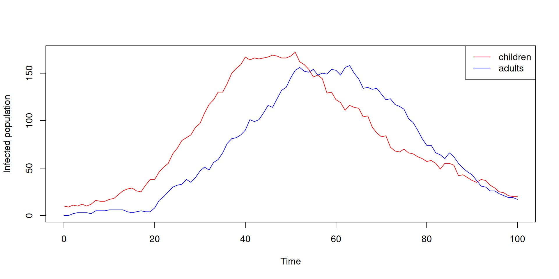
In the book: Arrays
Key features of arrays
- All arrays (whether state variable or parameter) need a
dimequation - No use of
i,jetc on LHS - indexing on the LHS is implicit - Support for up to 8 dimensions, with index variables
i,j,k,l,i5,i6,i7,i8 - Functions for reducing arrays such as
sum,prod,min,max- can be applied over entire array or slices
In the book: Arrays
Arrays: model with age and vaccine
sir_age_vax <- odin({
  # Equations for transitions between compartments by age group
  update(S[, ]) <- new_S[i, j]
  update(I[, ]) <- I[i, j] + n_SI[i, j] - n_IR[i, j]
  update(R[, ]) <- R[i, j] + n_IR[i, j]
  update(incidence) <- incidence + sum(n_SI)

  # Individual probabilities of transition:
  p_SI[, ] <- 1 - exp(-rel_susceptibility[j] * lambda[i] * dt) # S to I
  p_IR <- 1 - exp(-gamma * dt) # I to R
  p_vax[, ] <- 1 - exp(-eta[i, j] * dt)

  # Force of infection
  m <- parameter() # age-structured contact matrix
  s_ij[, ] <- m[i, j] * sum(I[j, ])
  lambda[] <- beta * sum(s_ij[i, ])

  # Draws from binomial distributions for numbers changing between
  # compartments:
  n_SI[, ] <- Binomial(S[i, j], p_SI[i, j])
  n_IR[, ] <- Binomial(I[i, j], p_IR)

  # Nested binomial draw for vaccination in S
  # Assume you cannot move vaccine class and get infected in same step
  n_S_vax[, ] <- Binomial(S[i, j] - n_SI[i, j], p_vax[i, j])
  new_S[, 1] <- S[i, j] - n_SI[i, j] - n_S_vax[i, j] + n_S_vax[i, n_vax]
  new_S[, 2:n_vax] <- S[i, j] - n_SI[i, j] - n_S_vax[i, j] + n_S_vax[i, j - 1]

  initial(S[, ]) <- S0[i, j]
  initial(I[, ]) <- I0[i, j]
  initial(R[, ]) <- 0
  initial(incidence, zero_every = 1) <- 0

  # User defined parameters - default in parentheses:
  S0 <- parameter()
  I0 <- parameter()
  beta <- parameter(0.0165)
  gamma <- parameter(0.1)
  eta <- parameter()
  rel_susceptibility <- parameter()

  # Dimensions of arrays
  n_age <- parameter()
  n_vax <- parameter()
  dim(S, S0, n_SI, p_SI) <- c(n_age, n_vax)
  dim(I, I0, n_IR) <- c(n_age, n_vax)
  dim(R) <- c(n_age, n_vax)
  dim(m, s_ij) <- c(n_age, n_age)
  dim(lambda) <- n_age
  dim(eta) <- c(n_age, n_vax)
  dim(rel_susceptibility) <- c(n_vax)
  dim(p_vax, n_S_vax, new_S) <- c(n_age, n_vax)
})
In the book: Arrays
Arrays: boundary conditions
Multiline equations can be used to deal with boundary conditions, e.g. we have
which we could also write as
or another way of writing this would be to use if ... else
In the book: Arrays
Dimensions
Dimensions can be hard-coded:
or can be soft-coded via parameters:
In the book: Arrays
Dimensions
Array parameters can have dimensions explicitly declared
or detected when the parameters are passed into the system - but a dim equation is needed where you must explicitly state the rank:
In the book: Arrays
Dimensions
Dimensions of one array can be declared as the same as the dimensions of another:
or dimensions of arrays that have the same dimensions can be declared collectively:
In the book: Arrays
Compilation error messages
Let’s revisit the stochastic SIR model, which compiles successfully:
sir <- odin({
  update(S) <- S - n_SI
  update(I) <- I + n_SI - n_IR
  update(R) <- R + n_IR
  update(incidence) <- incidence + n_SI

  p_SI <- 1 - exp(-beta * I / N * dt)
  p_IR <- 1 - exp(-gamma * dt)
  n_SI <- Binomial(S, p_SI)
  n_IR <- Binomial(I, p_IR)

  initial(S) <- N - I0
  initial(I) <- I0
  initial(R) <- 0
  initial(incidence, zero_every = 1) <- 0

  N <- parameter(1000)
  I0 <- parameter(10)
  beta <- parameter(0.2)
  gamma <- parameter(0.1)
})

sir
#>
#> ── <dust_system_generator: odin_system> ────────────────────────────────────────
#> ℹ This system runs in discrete time with a default dt of 1
#> ℹ This system has 4 parameters
#> → 'N', 'I0', 'beta', and 'gamma'
#> ℹ Use dust2::dust_system_create() (`?dust2::dust_system_create()`) to create a system with this generator
#> ℹ Use coef() (`?stats::coef()`) to get more information on parameters
In the book: Debugging
Compilation error messages
Now let’s remove the initial(R) equation
sir <- odin({
  update(S) <- S - n_SI
  update(I) <- I + n_SI - n_IR
  update(R) <- R + n_IR
  update(incidence) <- incidence + n_SI

  p_SI <- 1 - exp(-beta * I / N * dt)
  p_IR <- 1 - exp(-gamma * dt)
  n_SI <- Binomial(S, p_SI)
  n_IR <- Binomial(I, p_IR)

  initial(S) <- N - I0
  initial(I) <- I0
  initial(incidence, zero_every = 1) <- 0

  N <- parameter(1000)
  I0 <- parameter(10)
  beta <- parameter(0.2)
  gamma <- parameter(0.1)
})
#> Error in `odin()`:
#> ! Variables used in 'update()' do not have 'initial()' calls
#> ✖ Did not find 'initial()' calls for 'R'
#> → Context:
#> update(R) <- R + n_IR
#> ℹ For more information, run `odin2::odin_error_explain("E2003")`
In the book: Debugging
Compilation error messages
We can run odin_error_explain() with the corresponding error code as suggested (clickable in RStudio) for more information
odin_error_explain("E2003")
#>
#> ── E2003 ───────────────────────────────────────────────────────────────────────
#> Variables are missing initial conditions.
#>
#> All variables used in `deriv()` or `update()` require a corresponding entry in
#> `initial()` to set their initial conditions.  The error will highlight all
#> lines that have a `deriv()` or `update()` call that lacks a call to
#> `initial()`.  This can sometimes be because you have a spelling error in your
#> call to `initial()`.
#>
In the book: Debugging
Debugging
Here’s a model that compiles but has a bug
sir <- odin({
  update(S) <- S - n_SI
  update(I) <- I + n_SI
  update(R) <- R + n_IR
  update(incidence) <- incidence + n_SI

  p_SI <- 1 - exp(-beta * I / N * dt)
  p_IR <- 1 - exp(-gamma * dt)
  n_SI <- Binomial(S, p_SI)
  n_IR <- Binomial(I, p_IR)

  initial(S) <- N - I0
  initial(I) <- I0
  initial(R) <- 0
  initial(incidence, zero_every = 1) <- 0

  N <- parameter(1000)
  I0 <- parameter(10)
  beta <- parameter(0.2)
  gamma <- parameter(0.1)
})

sir
#> ── <dust_system_generator: odin_system> ────────────────────────────────────────
#> ℹ This system runs in discrete time with a default dt of 1
#> ℹ This system has 4 parameters
#> → 'N', 'I0', 'beta', and 'gamma'
#> ℹ Use dust2::dust_system_create() (`?dust2::dust_system_create()`) to create a system with this generator
#> ℹ Use coef() (`?stats::coef()`) to get more information on parameters
In the book: Debugging
Debugging
Let’s run it
The number of individuals in the R compartment has exceeded N!
In the book: Debugging
Debugging
You can stare at the code and hope to spot what’s wrong, but that can be like trying to find a needle in a haystack, especially for larger models.
So there are tools to help you:
- You can
print()the values of variables in your model as it runs - You can use the
browser()function in the same way as you would in R.
In the book: Debugging
Debugging: using print()
With print() we can tell it what to print and (optionally) conditions for when to print.
sir <- odin({
  update(S) <- S - n_SI
  update(I) <- I + n_SI
  update(R) <- R + n_IR
  update(incidence) <- incidence + n_SI

  p_SI <- 1 - exp(-beta * I / N * dt)
  p_IR <- 1 - exp(-gamma * dt)
  n_SI <- Binomial(S, p_SI)
  n_IR <- Binomial(I, p_IR)

  initial(S) <- N - I0
  initial(I) <- I0
  initial(R) <- 0
  initial(incidence, zero_every = 1) <- 0

  N <- parameter(1000)
  I0 <- parameter(10)
  beta <- parameter(0.2)
  gamma <- parameter(0.1)

  print("S + I: {S + I}, R: {R}", when = S + I + R > N && time > 5)
})
In the book: Debugging
Debugging: using print()
Then when we run it prints what we wanted with the times in square brackets:
This may help us spot that we’re not removing individuals from I when they move to R!
In the book: Debugging
Debugging: using browser()
With the browser() we need to declare the phase for inserting (deriv for ODE models, update for stochastic models) and optionally when to trigger it.
sir <- odin({
  update(S) <- S - n_SI
  update(I) <- I + n_SI
  update(R) <- R + n_IR
  update(incidence) <- incidence + n_SI

  p_SI <- 1 - exp(-beta * I / N * dt)
  p_IR <- 1 - exp(-gamma * dt)
  n_SI <- Binomial(S, p_SI)
  n_IR <- Binomial(I, p_IR)

  initial(S) <- N - I0
  initial(I) <- I0
  initial(R) <- 0
  initial(incidence, zero_every = 1) <- 0

  N <- parameter(1000)
  I0 <- parameter(10)
  beta <- parameter(0.2)
  gamma <- parameter(0.1)

  browser(phase = "update", when = S + I + R > N)
})
In the book: Debugging
Debugging: using browser()
When we try to run it will pause during evaluation:
You can list all the variables
In the book: Debugging
Debugging: using browser()
You can inspect values and perform calculations
In the book: Debugging
Debugging: using browser()
- Enter
corn, to continue until the next time thebrowser()is triggered
- If your model has a variable called
n, you would need to typemessage(n)to see its value - Enter
Qto immediately exit to the console with an error. - Run
dust_browser_continue()to cancel all futurebrowser()calls and continue running the model
In the book: Debugging
Next steps
- Get started fitting
odinmodels withmonty - Learn how to use
delay()for delay differential equations - Understand the order of events for discrete-time stochastic models
- For larger odin models, learn about packaging them