cases <-data()kappa <-parameter()cases ~NegativeBinomial(size = kappa, mean = incidence)
The distributions supported for likelihoods are the same as those supported for random draws - a full list with their names and parameterisations can be found here.
State space models
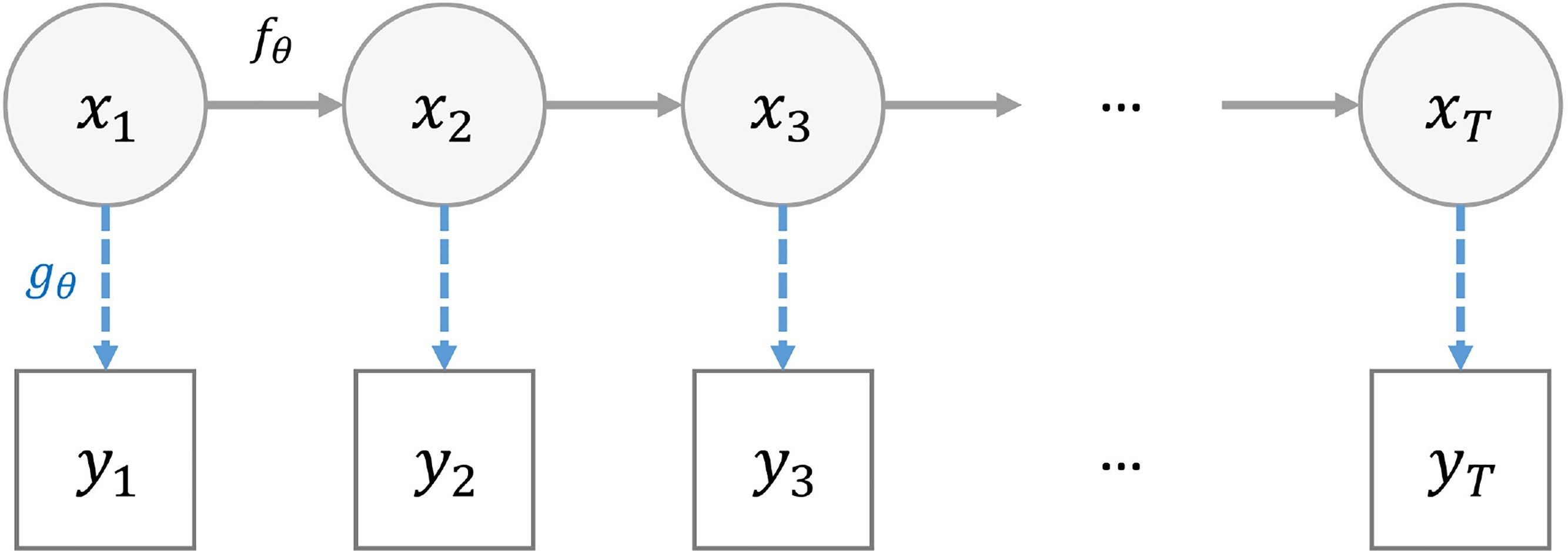
A state space model (SSM) is a mathematical framework for modelling a dynamical system.
It is built around two processes:
state equations that describes the evolution of some latent variables (also referred as “hidden” states) over time
observation equations that relates the observations to the latent variables.
Can you be more precise?
\(x_{t, 1 \leq t \leq T}\) the hidden states of the system
\(y_{t, 1 \leq t \leq T}\) the observations
\(f_{\theta}\) the state transition function
\(g_{\theta}\) the observation (likelihood) function
\(t\) is often time
\(\theta\) defines the model
Two common problems
Two common needs
“Filtering” i.e. estimate the hidden states \(x_{t}\) from the observations \(y_t\)
“Inference” i.e. estimate the \(\theta\)’s compatible with the observations \(y_{t}\)
Sequential Monte Carlo (SMC)
AKA, the (bootstrap) particle filter
Assuming a given \(\theta\), at each time step \(t\) it
generates \(X_{t+1}^N\) by using \(f_{\theta}(X_{t+1}^N|X_{t}^N)\) (the \(N\) particles)
calculates weights for the newly generated states based on \(g_{\theta}(Y_{t+1}|X_{t+1})\)
resamples the states to keep only the good ones
Allows to efficiently explore the state space by progressively integrating the data points
Produces a Monte Carlo approximation of \(p(Y_{1:T}|\theta)\) the marginal likelihood
Calculating likelihood: particle filtering
Calculating likelihood
data <-dust_filter_data(data, time ="time")filter <-dust_filter_create(sir, data = data, time_start =0,n_particles =200, dt =0.25)dust_likelihood_run(filter, list(beta =0.4, gamma =0.2))#> [1] -92.89566
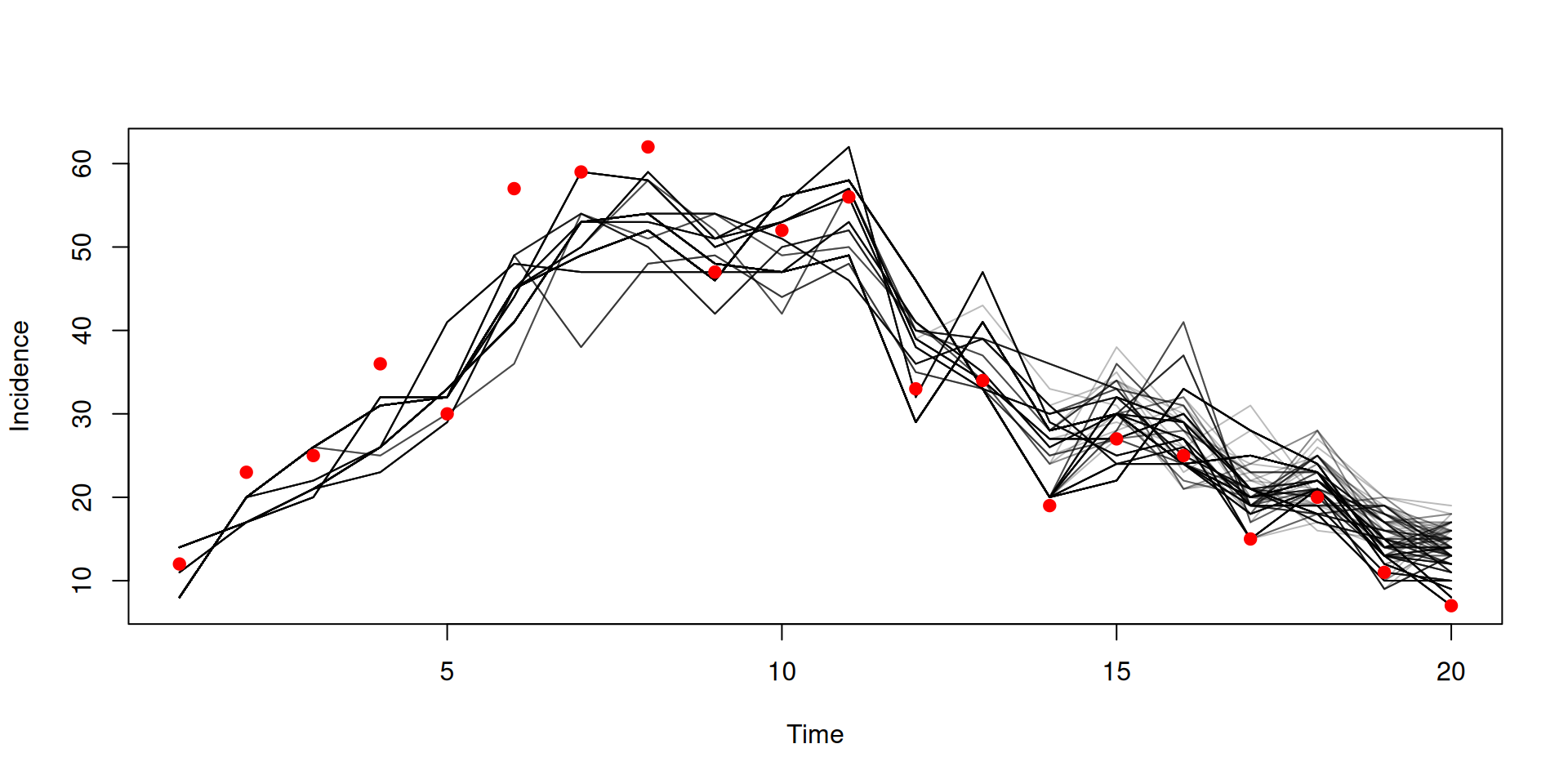
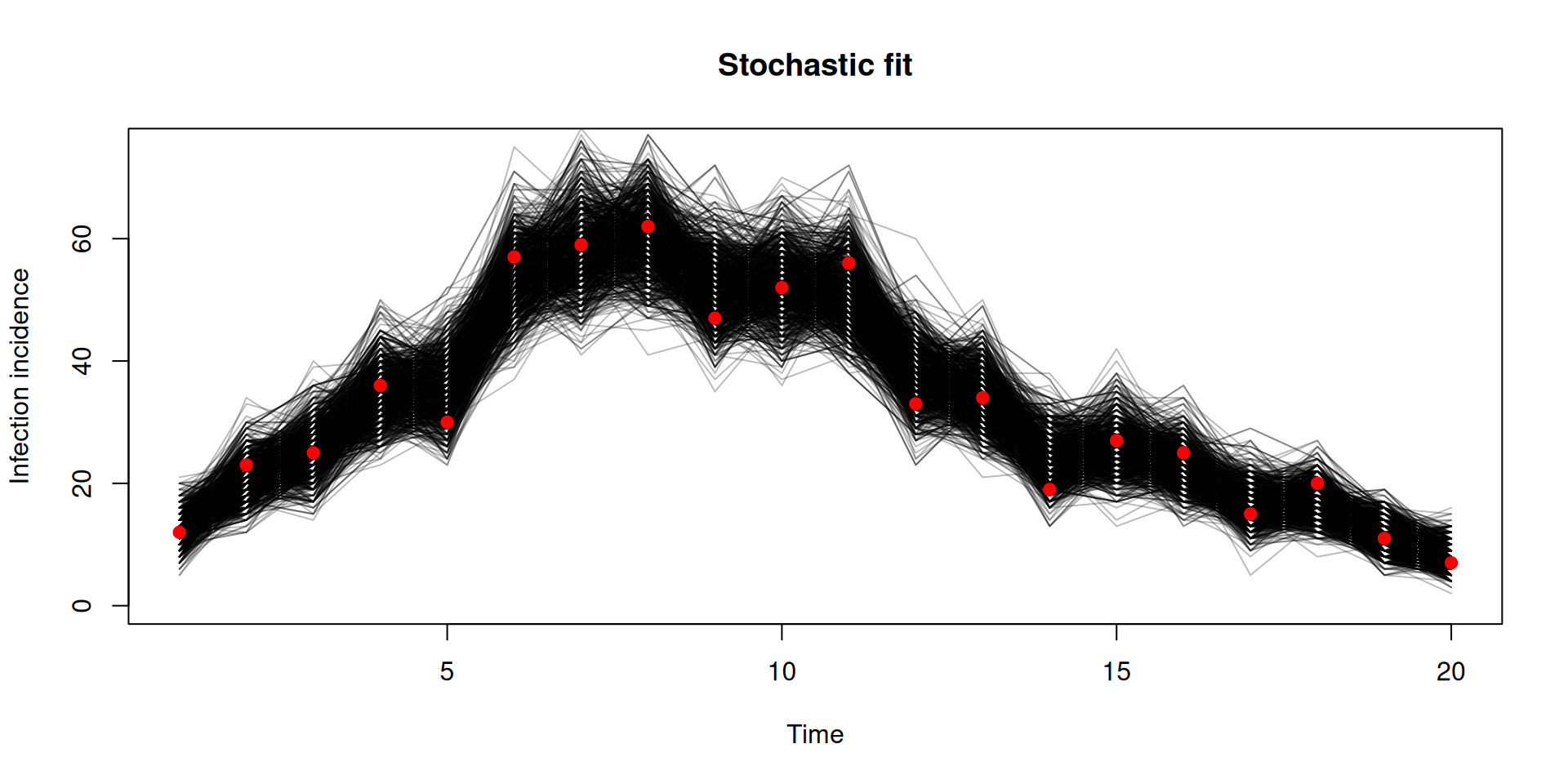
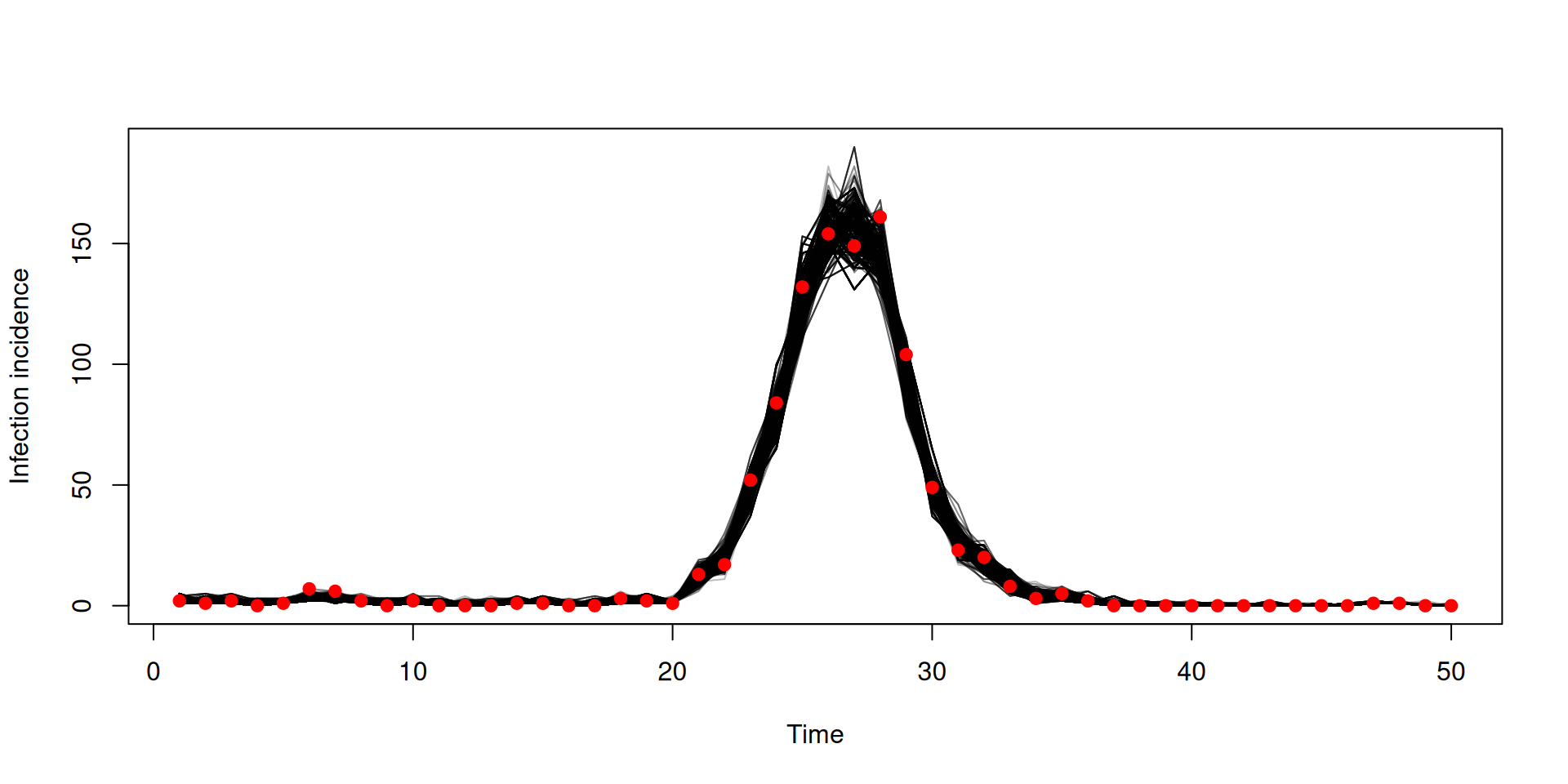
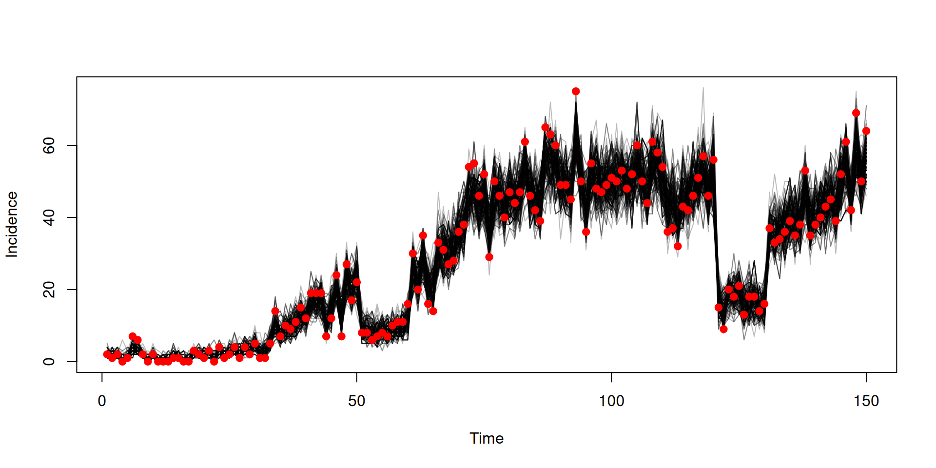
The system runs stochastically, and the likelihood is different each time:
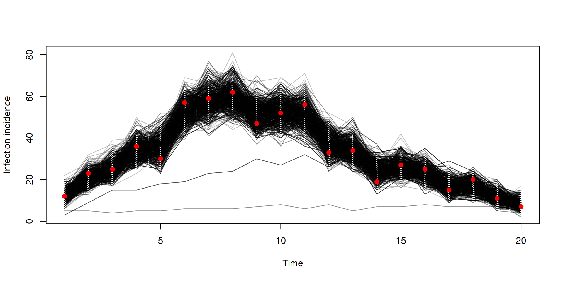
dust_likelihood_run(filter, list(beta =0.4, gamma =0.2),save_trajectories =TRUE)y <-dust_likelihood_last_trajectories(filter)y <-dust_unpack_state(filter, y)matplot(data$time, t(y$incidence), type ="l", col ="#00000044", lty =1,xlab ="Time", ylab ="Incidence")points(data, pch =19, col ="red")
Particle MCMC (PMCMC)
PMCMC is an algorithm which performs “filtering” and “inference”
A Markov Chain Monte Carlo (MCMC) method for estimating target distributions
MCMC explores the parameter space by moving randomly making jumps from one value to the next
In PMCMC, the marginal likelihood is estimated using a particle filter
One particle trajectory is selected randomly at the end of the particle filter
Particle MCMC
So we have a marginal likelihood estimator from our particle filter
How do we sample from beta and gamma?
We need:
to tidy up our parameters
to create a prior
to create a posterior
to create a sampler
“Parameters”
Our filter takes a list of beta and gamma, pars
it could take all sorts of other things, not all of which are to be estimated
some of the inputs might be vectors or matrices
Our MCMC takes an unstructured vector\(\theta\)
we propose a new \(\theta^*\) via some kernel, say a multivariate normal requiring a matrix of parameters corresponding to \(\theta\)
we need a prior over \(\theta\), but not necessarily every element of pars
Smoothing this over is a massive nuisance
some way of mapping from \(\theta\) to pars (and back again)
Parameter packers
Our solution, “packers”
packer <-monty_packer(c("beta", "gamma"))packer#> #> ── <monty_packer> ──────────────────────────────────────────────────────────────#> ℹ Packing 2 parameters: 'beta' and 'gamma'#> ℹ Use '$pack()' to convert from a list to a vector#> ℹ Use '$unpack()' to convert from a vector to a list#> ℹ See `?monty_packer()` for more information
Cope with vector- (or array-) parameters in \(\theta\) by declaring their dimensions as a named list passed in as the array argument. Fixed array parameters are just included in fixed.
packer <-monty_packer(c("beta", "gamma"),array =list(alpha =3, delta =c(2, 2)),fixed =list(eta =c(1, 3, 5)))packer#> #> ── <monty_packer> ──────────────────────────────────────────────────────────────#> ℹ Packing 9 parameters: 'beta', 'gamma', 'alpha[1]', 'alpha[2]', 'alpha[3]', 'delta[1,1]', 'delta[2,1]', 'delta[1,2]', and 'delta[2,2]'#> ℹ Use '$pack()' to convert from a list to a vector#> ℹ Use '$unpack()' to convert from a vector to a list#> ℹ See `?monty_packer()` for more informationpacker$unpack(c(0.2, 0.1, 0.31, 0.32, 0.33, 0.15, 0.16, 0.17, 0.18))#> $beta#> [1] 0.2#> #> $gamma#> [1] 0.1#> #> $alpha#> [1] 0.31 0.32 0.33#> #> $delta#> [,1] [,2]#> [1,] 0.15 0.17#> [2,] 0.16 0.18#> #> $eta#> [1] 1 3 5
The monty DSL
Working in a Bayesian framework, we will need to construct a prior distribution model for our parameters.
The distributions supported in the monty DSL are the same as those in odin2 - a full list with their names and parameterisations can be found here.
The monty DSL
The monty DSL creates a “monty model”
prior#> #> ── <monty_model> ───────────────────────────────────────────────────────────────#> ℹ Model has 2 parameters: 'beta' and 'gamma'#> ℹ This model:#> • can compute gradients#> • can be directly sampled from#> • accepts multiple parameters#> ℹ See `?monty_model()` for more information
The monty DSL
You can see the parameter names of the created model
prior$parameters#> [1] "beta" "gamma"
We can evaluate the (log) density for a given parameter vector (the order of parameters matches the above)
Which can be used for Hamiltonian Monte Carlo (HMC) - more support for this in future!
The monty DSL
In the monty DSL you can have the distribution of one parameter depend upon another
m <-monty_dsl({ a ~Normal(0, 1) b ~Normal(a, 1)})m#> #> ── <monty_model> ───────────────────────────────────────────────────────────────#> ℹ Model has 2 parameters: 'a' and 'b'#> ℹ This model:#> • can compute gradients#> • can be directly sampled from#> • accepts multiple parameters#> ℹ See `?monty_model()` for more information
The monty DSL
Order matters in the monty DSL - you cannot have the distribution of a parameter depend upon one defined later, so switching the order in our previous model results in an error
m <-monty_dsl({ b ~Normal(a, 1) a ~Normal(0, 1)})#> Error in `monty_dsl()`:#> ! Invalid use of variable 'a'#> → In expression#> b ~ Normal(a, 1)#> #> ℹ 'a' is defined later:#> a ~ Normal(0, 1)#> ℹ For more information, run `monty::monty_dsl_error_explain("E205")`
The monty DSL
You can use assignments to help make your code more understandable
m <-monty_dsl({ mu <-10 sd <-2 a ~Normal(mu, sd)})
these can also be used for intermediate calculations
m <-monty_dsl({ a ~Normal(0, 1) b ~Normal(0, 1) mu <- (a + b) /2 c ~Normal(mu, 1)})
The monty DSL
You can softcode values by passing them in as a list via fixed, e.g.
filter#> #> ── <dust_likelihood (odin_system)> ─────────────────────────────────────────────#> ℹ 4 state x 200 particles#> ℹ The likelihood is stochastic#> ℹ This system runs in discrete time with dt = 0.25#> ℹ Use coef() (`?stats::coef()`) to get more information on parameters
Combine a filter and a packer
packer <-monty_packer(c("beta", "gamma"))likelihood <-dust_likelihood_monty(filter, packer)likelihood#> #> ── <monty_model> ───────────────────────────────────────────────────────────────#> ℹ Model has 2 parameters: 'beta' and 'gamma'#> ℹ This model:#> • is stochastic#> ℹ See `?monty_model()` for more information
Posterior from likelihood and prior
Combine a likelihood and a prior to make a posterior
posterior <- likelihood + priorposterior#> #> ── <monty_model> ───────────────────────────────────────────────────────────────#> ℹ Model has 2 parameters: 'beta' and 'gamma'#> ℹ This model:#> • can be directly sampled from#> • is stochastic#> ℹ See `?monty_model()` for more information
(remember that addition is multiplication on a log scale)
Create a sampler
A diagonal variance-covariance matrix (uncorrelated parameters)
sampler <-monty_sampler_random_walk(vcv)sampler#> #> ── <monty_sampler: Random walk (monty_random_walk)> ────────────────────────────#> ℹ Use `?monty_sample()` to use this sampler#> ℹ See `?monty_random_walk()` for more information
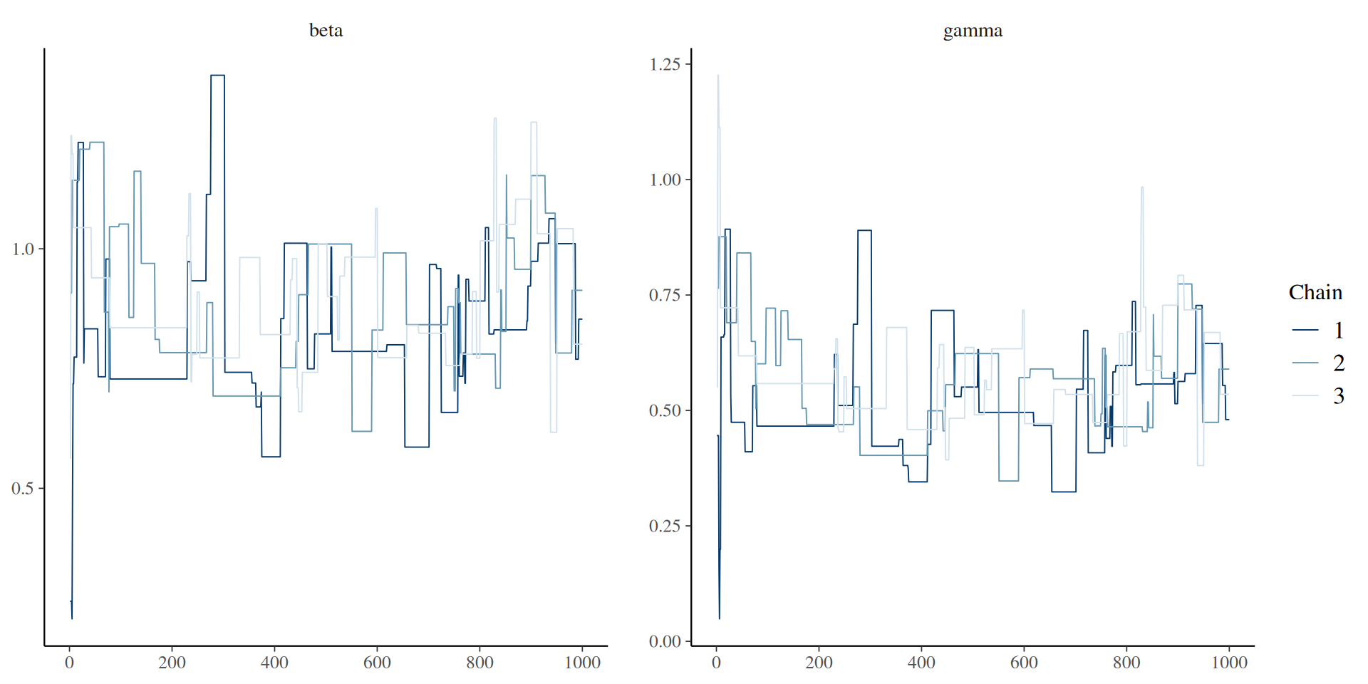
Let’s sample!
We will sample 4 chains, each with 1000 steps
samples <-monty_sample(posterior, sampler, 1000, n_chains =3)samples#> #> ── <monty_samples: 2 parameters x 1000 samples x 3 chains> ─────────────────────#> ℹ Parameters: 'beta' and 'gamma'#> ℹ Conversion to other types is possible:#> → ! posterior::as_draws_array() [package installed, but not loaded]#> → ! posterior::as_draws_df() [package installed, but not loaded]#> → ! coda::as.mcmc.list() [package installed, but not loaded]#> ℹ See `?monty_sample()` and `vignette("samples")` for more information
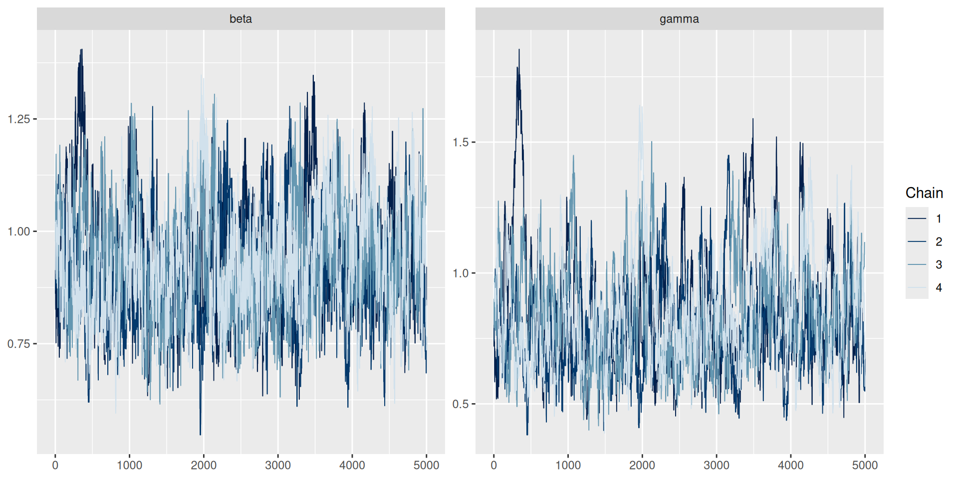
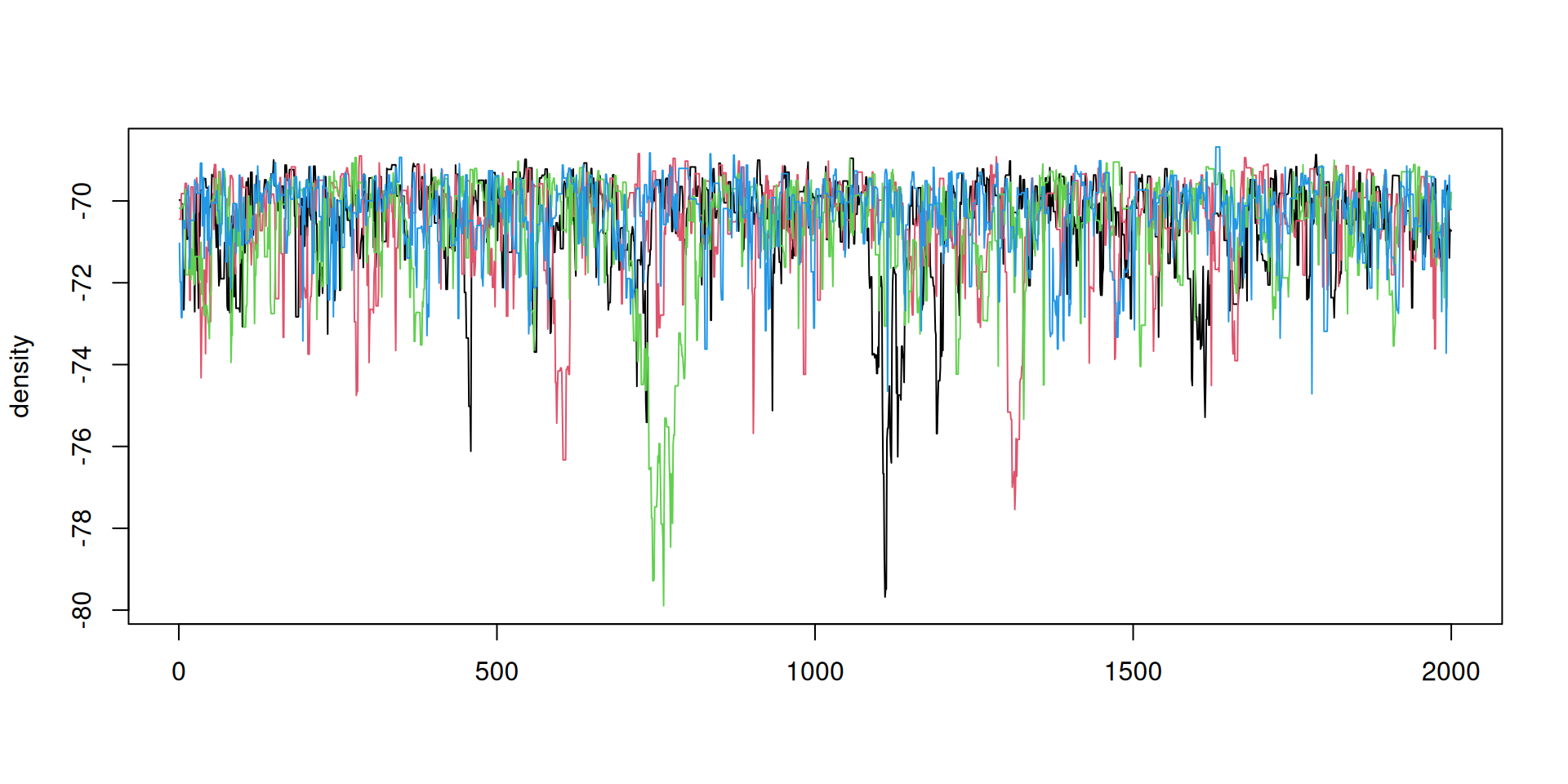
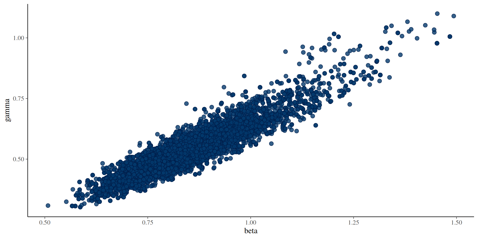
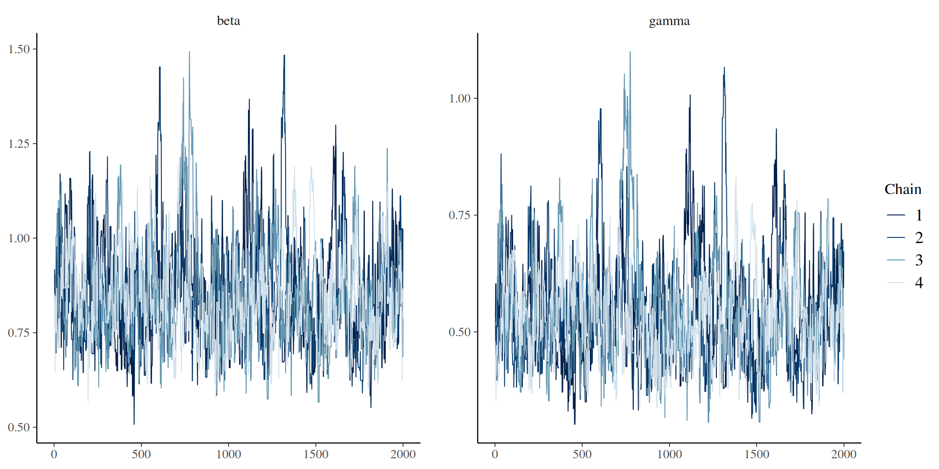
The result: diagnostics
Diagnostics can be used from the posterior package
Thinning while running faster and uses less memory
After running is more flexible (e.g. can plot full chains of parameters between running and thinning)
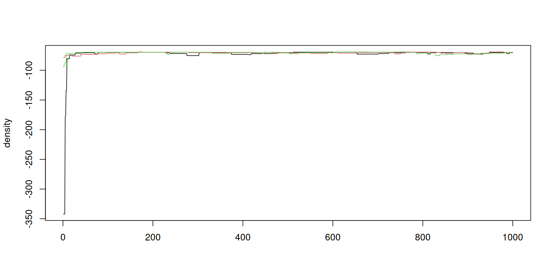
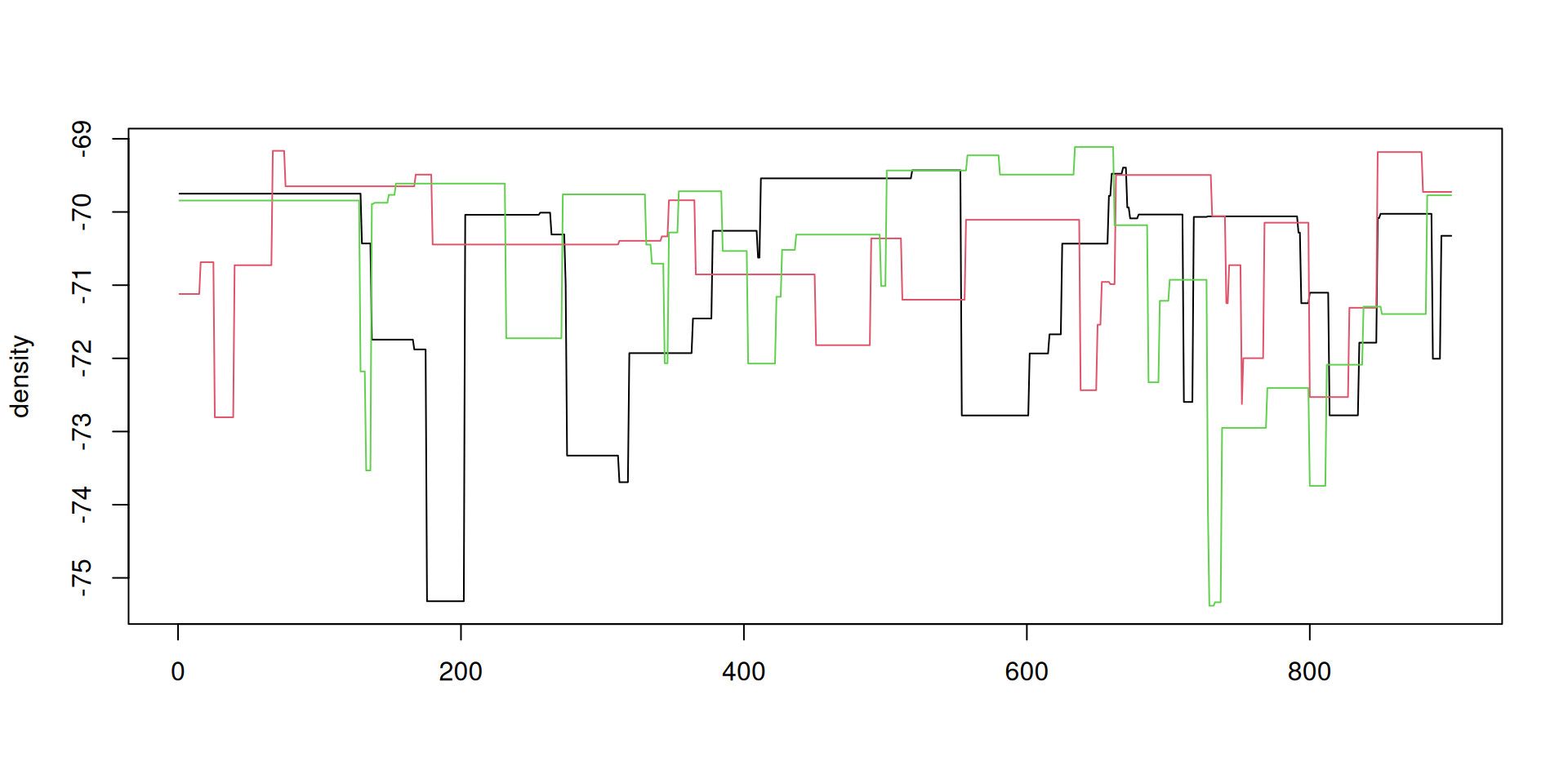
Dealing with sticky chains
Chains can get stuck when the variance of the marginal likelihood estimate is large
The chain has obtained a high-end marginal likelihood estimate at one parameter set and needs another high-end estimate at another parameter set to accept
You can increase the number of particles to reduce variance, but note this will take longer to run
In monty_sampler_random_walk you can rerun the particle filter at the current parameter set with the aim of calculating a lower estimate
rerun_every sets how often you rerun (rerun_every = 1000 means once every 1000 iterations)
rerun_random defines whether this occurs randomly (TRUE) or at fixed intervals (FALSE)
using the rerun comes at cost of some bias in the results
also some extra runtime cost (increasing the more frequently you rerun)
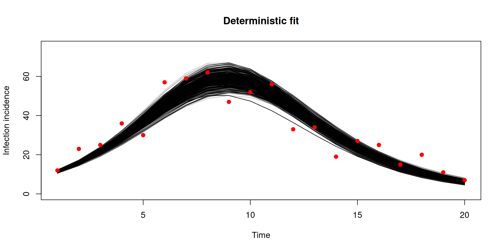
Deterministic models from stochastic
Stochastic models written in odin, can be run deterministically
Runs by taking the expectation of any random draws
This gives two models for the price of one
However it might not be suitable for all models
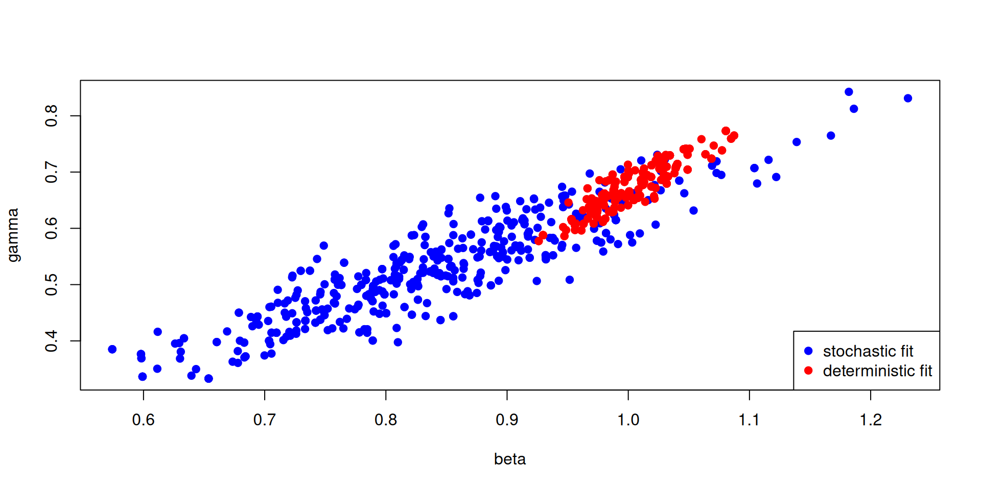
Fitting in deterministic mode
The key difference is to use dust_unfilter_create
unfilter <-dust_unfilter_create(sir, data = data, time_start =0, dt =0.25)
Note as this is deterministic it produces the same likelihood every time
posterior <- likelihood + priorposterior#> #> ── <monty_model> ───────────────────────────────────────────────────────────────#> ℹ Model has 3 parameters: 'gamma', 'beta[1]', and 'beta[2]'#> ℹ This model:#> • can be directly sampled from#> • is stochastic#> • has an observer#> ℹ See `?monty_model()` for more information
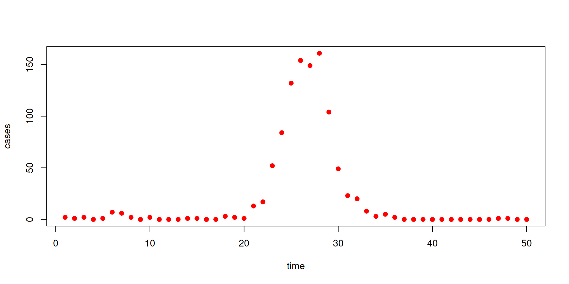
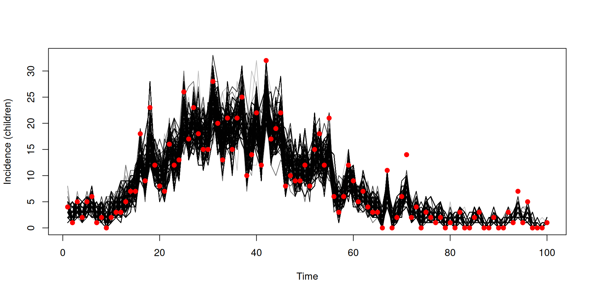
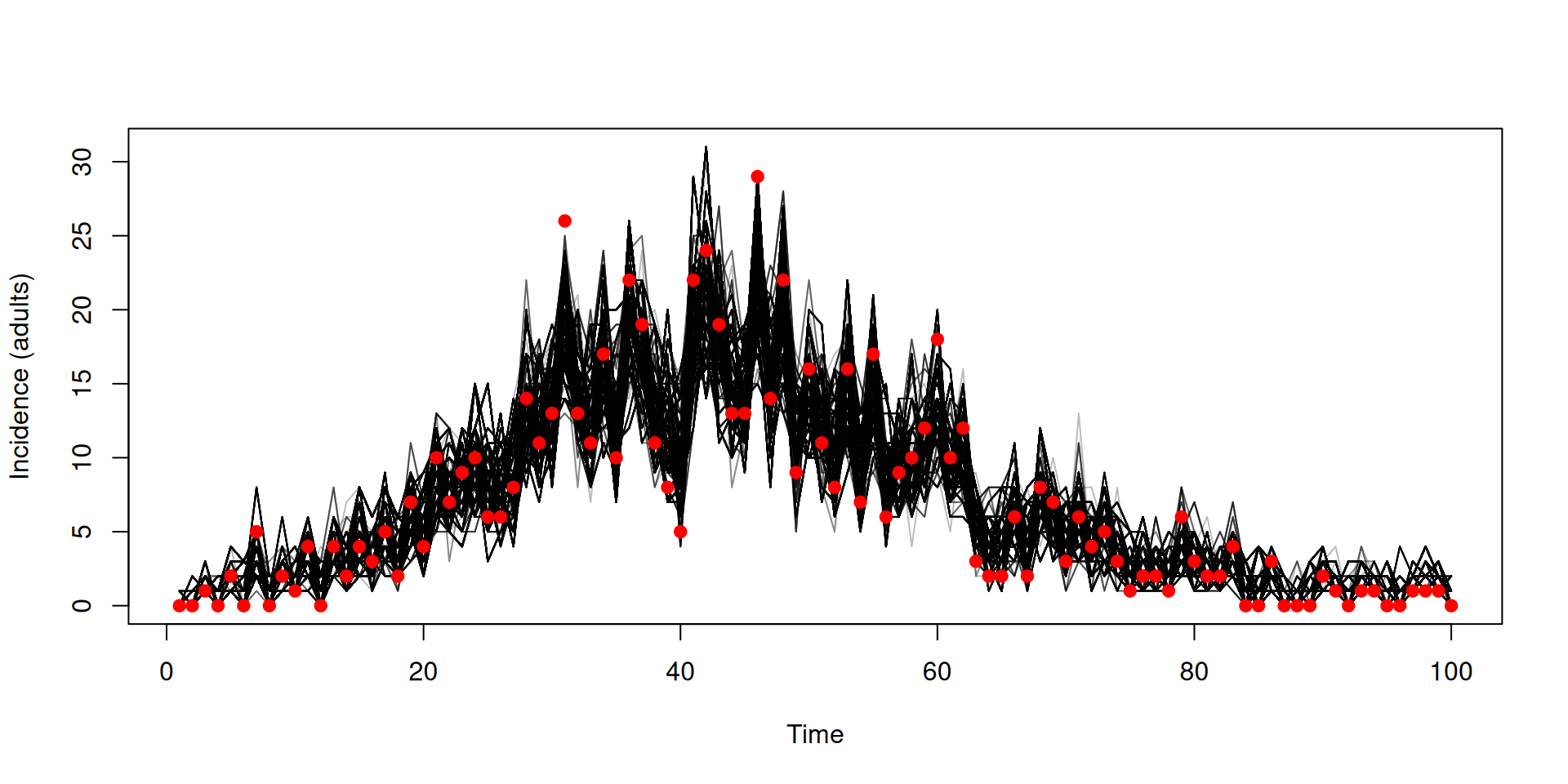
Let’s think of the cases data at each time point as a vector of length 2 (for the 2 age groups)
Fitting to vector/array data
We’ll fit these data to a model with age stratification
sir_age <-odin({# Equations for transitions between compartments by age groupupdate(S[]) <- S[i] - n_SI[i]update(I[]) <- I[i] + n_SI[i] - n_IR[i]update(R[]) <- R[i] + n_IR[i]update(incidence[]) <- incidence[i] + n_SI[i]# Individual probabilities of transition: p_SI[] <-1-exp(-lambda[i] * dt) # S to I p_IR <-1-exp(-gamma * dt) # I to R# Calculate force of infection# age-structured contact matrix: m[i, j] is mean number# of contacts an individual in group i has with an# individual in group j per time unit m <-parameter()# here s_ij[i, j] gives the mean number of contacts an# individual in group i will have with the currently# infectious individuals of group j s_ij[, ] <- m[i, j] * I[j]# lambda[i] is the total force of infection on an# individual in group i lambda[] <- beta *sum(s_ij[i, ])# Draws from binomial distributions for numbers# changing between compartments: n_SI[] <-Binomial(S[i], p_SI[i]) n_IR[] <-Binomial(I[i], p_IR)initial(S[]) <- S0[i]initial(I[]) <- I0[i]initial(R[]) <-0initial(incidence[], zero_every =1) <-0 S0 <-parameter() I0 <-parameter() beta <-parameter(0.2) gamma <-parameter(0.1) n_age <-parameter()dim(S, S0, n_SI, p_SI, incidence) <- n_agedim(I, I0, n_IR) <- n_agedim(R) <- n_agedim(m, s_ij) <-c(n_age, n_age)dim(lambda) <- n_age## Likelihood cases <-data()dim(cases) <- n_age cases[] ~Poisson(incidence[i])})
Fitting to vector/array data
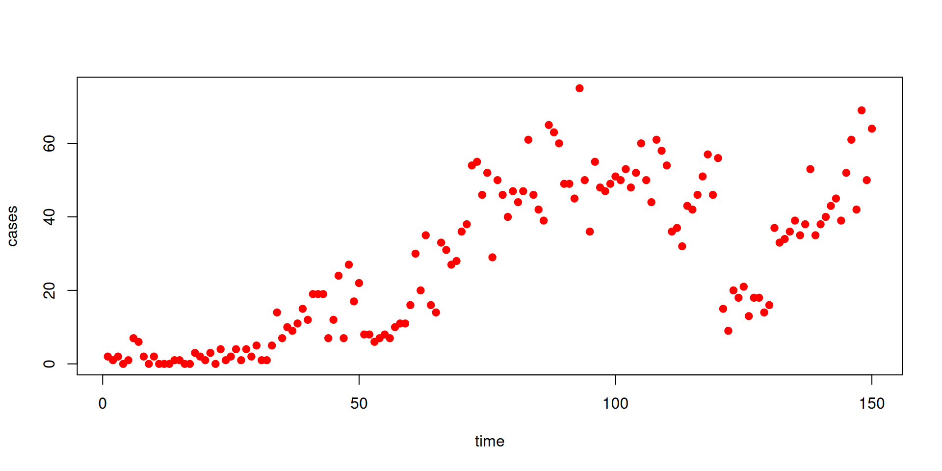
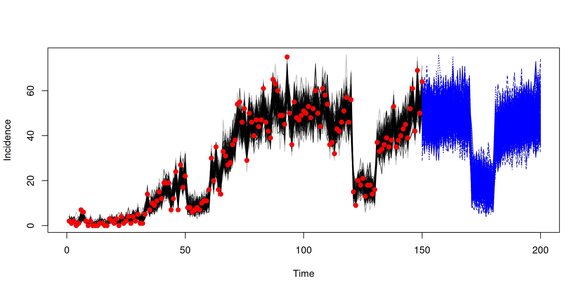
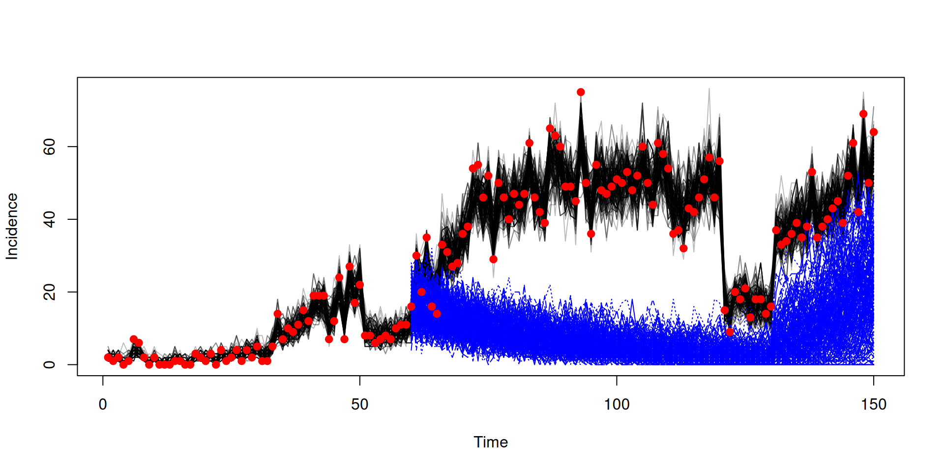
We are treating the data cases as a vector that relates to incidence from the model
y <-dust_unpack_state(filter, samples$observations$trajectories)incidence <-array(y$incidence, c(150, 200))matplot(data$time, incidence, type ="l", col ="#00000044", lty =1,xlab ="Time", ylab ="Incidence")points(data, pch =19, col ="red")
matplot(data$time, incidence, type ="l", col ="#00000044", lty =1,xlab ="Time", ylab ="Incidence")matlines(t, t(y$incidence), col ="blue")points(data, pch =19, col ="red")