SLiM: review and profiling for malaria models
Shazia Ruybal-Pesántez
Last updated: 30 Mar 2023
Source:vignettes/SLiM_review.Rmd
SLiM_review.RmdBackground
This notebook documents the review of the forward genetic simulation
tool SLiM (Benjamin C. Haller and Messer 2019, 2019; Benjamin C.
Haller and Messer 2016; Messer 2013). We are testing whether this
tool can be used as a part of the SIMPLEGEN pipeline. Some key
advantages of SLiM that would be beneficial for our purposes is the
ability to simulate haploid genomes and because of its well-integrated
tskit tree structure format for genetic data, which is
already debugged and working seamlessly with simulation output from
SLiM. However we will test whether SLiM is suitable for large population
sizes and to build an appropriate malaria model (eg Ross-MacDonald).
(Potentially other things to test as well)
Main aims:
- Literature review of SLiM for malaria simulations (have people used this tool? if not, maybe there is a reason why…)
- Attempt to build a simple P. falciparum genetic model
- Attempt to build a simple Ross-MacDonald host-vector model
- Profile SLiM for simulations with large population sizes and large generation/run times
Brief overview of SLiM
The majority of papers citing SLiM use SLiM for simulations of human genomics because of the flexibility to simulate one or more genomic elements and different types of mutations (e.g. beneficial, deleterious, neutral) simultaneously under realistic evolutionary conditions (mutation and recombination rates). In addition, the SLiM manual (>700 pages) provides a comprehensive resource on how to customize SLiM, details on the coding language Eidos, ready-made “recipes” for common scenarios (eg selective sweeps, bottlenecks etc) and the interactive GUI enables visualization of the genome in real-time as simulations are running. For example, a particular beneficial mutation can be seen increasing in frequency until fixation. SLiM also provides useful profiling reports that document CPU and memory usage, and show the breakdown of usage based on distinct parts of the code. SLiM can be run in the interactive GUI or via the command line.
Outputs from SLiM
SLiM allows several output formats and also supports custom scripting
using the Eidos language. This is possible not only for model
specifications/customization but also for the model output (eg using
paste() or cat() to build output data
frames).
Some of the output possibilities in SLiM include (but not limited to):
outputGenome(): entire genome informationoutputVCF(): nucleotide VCF format (note based on a sample of individuals and need to consideroutputMultiallelicsparameter)outputMutations()oroutputFixedMutations(): information on explicitly tracked or fixed mutations, respectivelyoutputPedigree(): pedigree tracking can be turned on and the simulation will keep track of every individual, their parents, grandparents etc. Pedigree output requires custom Eidos scripting (as far as I can tell).outputTreeSeq(): output tree-sequence recording intskit-format.trees(note much more efficient and more compact than eg VCF). Worth noting thatmsprimecan write vcf files from.trees
Tree-sequence recording in SLiM
One of the key features of SLiM is the ability to output genetic data
in tree-sequence format, .trees (Kelleher et al. 2018) to track population
history and true local ancestry. This type of output then enables
seamless integration with tskit
and msprime
and can be analyzed downstream with Python and pyslim,
a Python API developed specifically for interchangeability between SLiM,
tskit, msprime etc. Similarly R can be used
downstream and there are also specific R packages such as {slendr} developed specifically for
this (see (Petr et al. 2022)). There are
several advantages to tree-sequence recording such as but not limited to
(for more details see (Benjamin C. Haller et al.
2019) and SLiM manual Chapter 1.7 and 17):
Overlaying neutral mutations: forward simulations can be run without neutral mutations to significantly increase computational efficiency and speed (by order of magnitude or more if a model contains many neutral mutations). The neutral mutations can then be overlaid only on “pruned” trees using
msprime.-
Increase efficiency of burn-in: forward simulations can be run with no neutral burn-in (ie empty genomes) and then using “recapitation” the ancestry is reconstructed using the coalescent of only the ancestry trees present at the end. Neutral mutations can then be overlaid after the fact.
- Note: it is also possible to seamlessly move between coalescent and
forward simulations, eg burn-in can be simulated in
msprimewithout mutations, then the.treesfile can be used in SLiM as the starting state (ie non-neutral simulations can be simulated forwards in time). Mutations can be overlaid either withmsprimeor after the forwards simulation as described above.
- Note: it is also possible to seamlessly move between coalescent and
forward simulations, eg burn-in can be simulated in
Direct analysis of ancestry trees: when the ancestry pattern is of interest (not the pattern of neutral mutations), inferences may be more robust for this purpose by using the recorded tree sequence (ie every possible mutational history event given true history of inheritance/recombination)
Multi-species models
The most recent release of SLiM, 4 (Benjamin C. Haller and Messer 2022) allows multi-species simulations and the ability for custom scripting to deal with spatial landscapes (continuous-space models). This version now also allows simulation of “non-genetic” species, enabling modeling of ecological scenarios (eg fox and mouse), with the flexibility to simulate genetics for one or more species or none, but also allowing interactions between them as needed. We explore this possibility for building a vector-host model (see Profiling SLiM: basic Ross-Macdonald epidemiological model of malaria section below).
Brief literature review of SLiM for Plasmodium spp
Out literature review identified only three publications where SLiM was used for simulations in malaria, described below:
Henden et al, PLOS Genetics 2018, Identity-by-descent analyses for measuring population dynamics and selection in recombining pathogens (Henden et al. 2018)
- SLiM was used to simulate SNP data and hard sweeps with an evolutionary model appropriate for P. falciparum to test whether their IBD method was able to detect the expected positive selection signatures. The simulations were also used to benchmark the IBD method compared to integrated haplotype score (iHS) and extended haplotype homozygosity (EHH) in detecting these signatures of selection.
- Parameters used:
Constant effective population size of P. falciparum of 100,000 (as per (Hughes and Vierra 2001))
Mutation rate of 1.7x10⁻⁹ per base pair per generation (as per (Bopp et al. 2013))
Recombination rate of 7.4 x 10⁻⁷ per base pair per generation (or 13.5 kb/cM as per (Miles et al. 2016))
Generation time: 400,000 generations
Genomic element: Chromosome 12, 2.2Mb
Sample of 10,000 haplotypes randomly drawn to undergo hard and soft sweeps (see Materials and Methods of paper for more details). Note: from methods text “We note that it would have been desirable to run the simulation over more generations [20], however this was not computationally feasible with the forward simulator.”
Tennessen and Duraisingh, Molecular Biology and Evolution 2020, Three Signatures of Adaptive Polymorphism Exemplified by Malaria-Associated Genes (Tennessen and Duraisingh 2020)
- SLiM was used to simulate human genetics and explore malaria-associated balancing selection signatures.
- Parameters used (1000 replicate simulations for each set of params):
Population size: 10,000 individuals
Mutation rate: 1x10⁻⁷ or 2x10⁻⁷
Recombination rate: 0.01 or 0.001 (population-scaled)
Genomic element: 10,001 bp
-
Polymorphisms neutral except for overdominant balanced polymorphism in the center (dominance coefficient 1e6; selection coefficient 1e-8 or dominance coeff 1.1; selection coeff 0.1)
- also ran simulations where all polymorphisms selectively neutral
Generation time: 50000, 100000, 200000
Hamid et al, eLife 2021, Rapid adaptation to malaria facilitated by admixture in the human population of Cabo Verde (Hamid et al. 2021)
SLiM was used to simulate human genetics and explore adaptation to malaria in admixed human populations using tree-sequence recording.
-
Parameters used (the combinations of which produced 8 different demographic scenarios - 1000 replicate simulations for each):
-
Population size: 1000 or 10,000
either constant population size or exponential growth at rate 0.05 per generation
either single pulse of admixture at start of simulation or continuous admixture at 1% total new migrants per generation
Generation time: 20
Genomic element: human chr1
Admixture from two source pops forming a third admixed pop
-
Building a simple model for P. falciparum genetics in SLiM
Given the limited application of SLiM in the malaria literature, and even more so for simulating Plasmodium spp, we replicated the model of Henden et al. (Henden et al. 2018) with a few modifications (detailed below) to gauge the simulation run times in SLiM.
Model details
We implemented a simple Wright-Fisher model in SLiM with only neutral mutations. The parameters we used are indicated below:
-
Effective population size, Ne= 100,000
- An acceptable range in the literature is reported as: 104-106 as per (Hughes and Vierra 2001)
-
Mutation rate: 1.7x10⁻⁹
This mutation rate is often used, 1.7x10⁻⁹ per base pair per generation (range: 1.7-3.2x10⁻⁹ as per (Bopp et al. 2013)).
However it is worth noting there are other studies documenting average mutation rate of 2x10⁻¹⁰ per base pair per generation, where a generation corresponds to a 48hr intra-erythrocytic asexual cycle (range: 3.82-4.28x10⁻¹⁰ as per (Claessens et al. 2014; Hamilton et al. 2016)). Mutation rate estimates are reviewed in Anderson et al (T. J. C. Anderson et al. 2016), see Table 4. In this paper, mutation rates are converted from a per cycle rate to a generation mutation rate, assuming 2-month generation time for duration of entire parasite life cycle, ie mosquito-human-mosquito. In this model we did not convert between generations and cycles, but this is worth considering in future if Plasmodium genetics are to be simulated appropriately
-
Recombination rate: 7.4x10⁻⁷ and assumed to be uniform across genome
- This recombination rate (cross-over) average of 7.4x10⁻⁷ or 13.5kb/cM (95%CI: 12.7-14.3) is reported in (Miles et al. 2016) (note: IsoRelate and hmmIBD implement the same recombination rate)
Genomic element: 2.2Mb (corresponding to P. falciparum chromosome 12 as per Henden et al)
Generation time: 400,000
Results and considerations
This simulation took an extremely long time to run (>3 days), acknowledging that the generation time was also long given it is more representative of a “burn-in” period rather than comparative simulations to what we will perform in SIMPLEGEN. From this exercise we note that SLiM can potentially be used for simulating a P. falciparum burn-in where, for instance, neutral mutations are overlaid after the fact (as described in Tree-sequence recording in SLiM). This output could be saved and used as a initial state for further forward simulation. SLiM can thus potentially be used to generate a “null” P. falciparum population with realistic sequence variation if an appropriate evolutionary history can be simulated. This would require more robust parameterization of Plasmodium genetics than what we simulated above.
Profiling SLiM: basic Ross-Macdonald epidemiological model of malaria
One of the key features of SIMPLEGEN is the ability to generate transmission records) where the transmission history of every infection is tracked and recorded (eg. human to mosquito transmission, followed by the next blood meal and transmission to another human, etc.). We are not interested in simulating genetics in SLiM per se, rather we are interested in the ability to generate tree-sequence recording of such a transmission history. We explore the possibility of implementing a simple Ross-Macdonald epidemiological model with no genetics in SLiM with tree-sequence recording below.
Model details
To build the Ross-Macdonald epidemiological model we use the multi-species functionality of SLiM to create both human and mosquito species. There are two equations that drive the dynamics in this simple model, as described by Aron and May (Aron and May 1982) (also see Smith et al. for a comprehensive review of Ross-Macdonald model theory and an overview of the model notation in Box 2 (Smith et al. 2012)). The first equation describes the change in human states:
\(\frac{dx}{dt} = mabx(1-x)-rx\),
where \(x\) is the number of infected humans, \(m\) is the ratio of mosquitoes to humans, \(a\) is the human blood feeding rate or proportion of mosquitoes that feed each day, \(b\) is the proportion of bites by infectious mosquitoes that infect a human, and \(r\) is the daily rate each human recovers from infection. The parameter \(ma\) is a measurable parameter corresponding to the human biting rate or the number of bites by vectors per humans per day. The second equation describes the change in mosquito states:
\(\frac{dz}{dt} = ax(1-z)-gz\),
where \(z\) is the number of infected mosquitoes, and \(g\) is the instantaneous death rate of mosquitoes.
Both humans and mosquitoes can transition from a susceptible to infected state and the population sizes of humans and mosquitoes are fixed. We used the following parameters (Table 1), with fixed fixed parameters indicated in bold:
Table 1. Simulation parameters for Ross-Macdonald implementation in SLiM
| Parameter | Description | Value | Notes |
|---|---|---|---|
| \(N_h\) | Number of human hosts | 1000, 10000, 100000, 1000000 | |
| \(N_v\) | Number of mosquito vectors | 50000, 500000, 5000000 | |
| \(ma\) | Human biting rate | 0.1 | This is equivalent to a mosquito biting every 10 days |
| \(r\) | Human infection clearance rate | 0.05 | This is equivalent to a human clearing their infection every 3 weeks |
| \(g\) | Mosquito mortality rate | 0.2 | This is equivalent to every mosquito having a probability of survival of 0.8 (see (Hendry, Kwiatkowski, and McVean 2021)) |
It is worth noting that the aim was not to fully parameterize the model itself as we were more interested in profiling SLiM simulations in terms of CPU time and memory usage.
We seed the model at day 50 with 100 infected individuals and the let simulation run for 5, 10, 25 or 50 years for the following combinations of \(N_h\) and \(V_h\):
\(N_h\)= 1000; \(V_h\)= 50,000
\(N_h\)= 10,000; \(V_h\)= 500,000
\(N_h\)= 100,000; \(V_h\)= 5,000,000
\(N_h\)= 1,000,000; \(V_h\)= 5,000,000 (note: for the 25 and 50 year simulations we did not run this)
There are no genetics included in this model but according to the SLiM manual, strain properties infecting an individual could in theory be “tracked” throughout the time series. Another possibility would be to have a three-species model where Plasmodium spp is modeled including host-parasitoid interactions (eg. parasite density, parasite strain ID tracking, for details see SLiM manual Chapters 19.3 and 19.4). However, for our purposes even the multi-species SLiM model is not suitable for tree-sequence recording outputs because this functionality is only available for tracking within one species. In our case, the ability to record tree “branches” between mosquito to human and human to mosquito are necessary to fully capture the ancestral “infection” tree for downstream genetic analyses.
Results of profiling the model
We tested the speed of the simulations by varying human and mosquito populations sizes (1e3 to 1e6 and 5e4 to 5e6, respectively), as well as the number of years the simulation was run (5, 10, 25 and 50 years) as described in Model details.
By using the clock feature on the SLiM GUI we can profile each simulation run, which outputs useful information like CPU time elapsed during the run (we are interested in the “Elapsed wall clock time inside SLiM core (corrected)”, which is measured in seconds) as well as average memory usage across all “ticks” or generations (we are interested in the “Average tick SLiM memory use”, which is measured in megabytes).
profile_stats <- data.frame(test= c("H=1e3, M=5e4", "H=1e4, M=5e5", "H=1e5, M=5e6", "H=1e6, M=5e6",
                                    "H=1e3, M=5e4", "H=1e4, M=5e5", "H=1e5, M=5e6",
                                    "H=1e3, M=5e4", "H=1e4, M=5e5", "H=1e5, M=5e6",
                                    "H=1e3, M=5e4", "H=1e4, M=5e5", "H=1e5, M=5e6"),
                            pop_size_humans = c(1e3, 1e4, 1e5, 1e6,
                                                1e3, 1e4, 1e5,
                                                1e3, 1e4, 1e5,
                                                1e3, 1e4, 1e5),
                            pop_size_mosquito = c(5e4, 5e5, 5e6, 5e6,
                                                  5e4, 5e5, 5e6,
                                                  5e4, 5e5, 5e6,
                                                  5e4, 5e5, 5e6),
                            years = c(5, 5, 5, 5,
                                      10, 10, 10,
                                      25, 25, 25,
                                      50, 50, 50),
                            cpu_time = c(19.12, 270.03, 2440.64, 6544.94,
                                         38.36, 501.69, 5210.31,
                                         117.17, 1188.88, 22804.75,
                                         200.18, 2715.99, 41697.93),
                            avg_memory = c(29.02, 192.06, 1800, 2100,
                                           29.03, 192.11, 1800,
                                           29.03, 192.14, 1800,
                                           29.03, 192.14, 1800))
We found that the simulation run times were extremely slow, especially for human population sizes above 1000 (Figure 1). Even for 5 year simulations the CPU time required was between 4.5 to 109 minutes when the human population size was 10,000 up to the 1,000,000 value tested. The average memory usage was consistent regardless of simulation run time, but increased by an order of magnitude in line with increases in human population size (see Figure 1, or Figure 2 for interactive plot). When varying the mosquito population sizes we found similar trends as for increases in human population sizes (Figure 3).
(profile_stats %>%
  ggplot(aes(x = pop_size_humans, y = cpu_time/60, group = factor(years), color = factor(years))) +
    geom_point() +
    geom_line() +
    scale_x_continuous(breaks = scales::pretty_breaks(n=6)) +
    scale_y_continuous(breaks = scales::pretty_breaks(n=10)) +
    scale_color_manual(values = c("hotpink3", "goldenrod3", "lightblue3", "olivedrab3")) +
    xlim(0, 1e5) +
    labs(x = "Human population size",
         y = "CPU time (in minutes)",
         color = "Simulation run time (in years)",
         title = "Simple Ross-Macdonald model") +
    theme_minimal() +
    theme(legend.position = "none")) +

(profile_stats %>%
  ggplot(aes(x = pop_size_humans, y = avg_memory, group = factor(years), color = factor(years))) +
  geom_point() +
  geom_line(alpha=0.5) +
  scale_y_continuous(breaks = scales::pretty_breaks(n=5)) +
  scale_color_manual(values = c("hotpink3", "goldenrod3", "lightblue3", "olivedrab3")) +
  xlim(0, 1e5) +
  labs(x = "Human population size",
       y = "Average memory used (in megabytes)",
       color = "Simulation run time (in years)") +
  theme_minimal()) +

  plot_layout(guides = "collect")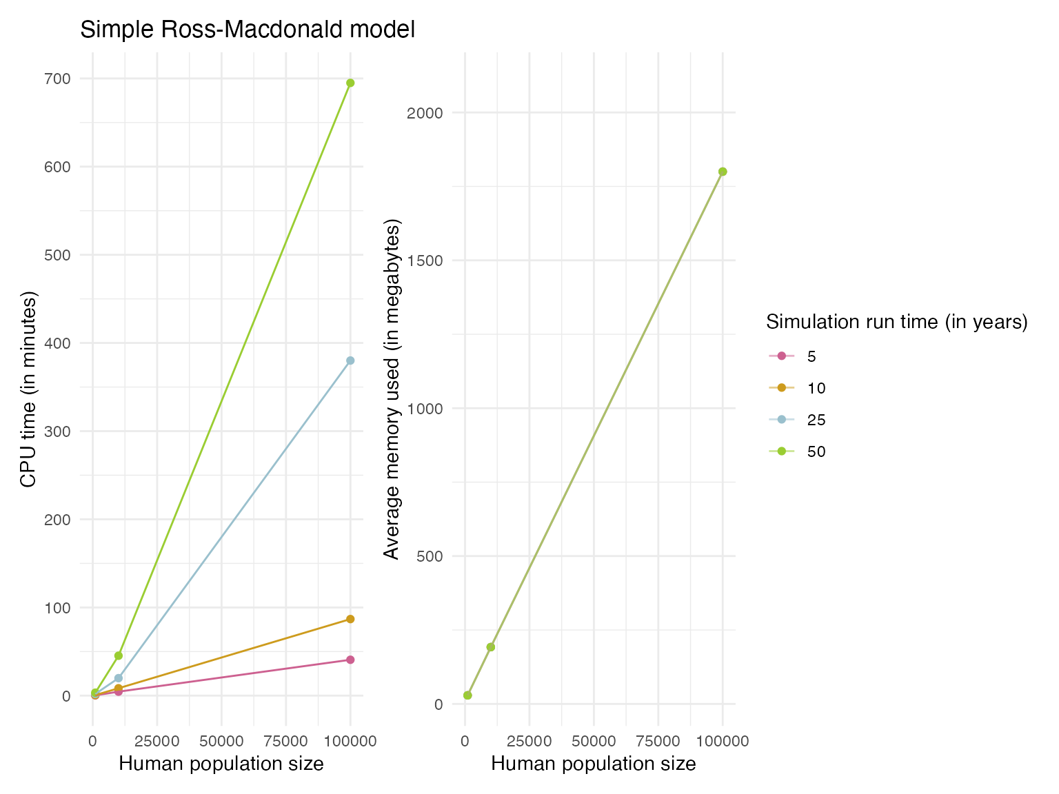
Figure 1. The profiling results showing the CPU times and memory usage for simulation runs with varying human population sizes
ggplotly(profile_stats %>%
  ggplot(aes(x = pop_size_humans, y = cpu_time/60, group = factor(years), color = factor(years))) +
    geom_point() +
    geom_line() +
    scale_y_continuous(breaks = scales::pretty_breaks(n=10)) +
    scale_color_manual(values = c("hotpink3", "goldenrod3", "lightblue3", "olivedrab3")) +
    xlim(0, 1e5) +
    labs(x = "Human population size",
         y = "CPU time (in minutes)",
         color = "Simulation run time (in years)",
         title = "Simple Ross-Macdonald model") +
    theme_minimal())
Figure 2. An interactive plot showing the profiling results for simulation runs with varying human population sizes
(profile_stats %>%
    filter(test != "H=1e6, M=5e6") %>%  # remove the test with human n=1e6 and m=5e6 as skews the trend visualization since two points have same mosq pop size
  ggplot(aes(x = pop_size_mosquito, y = cpu_time/60, group = factor(years), color = factor(years))) +
    geom_point() +
    geom_line() +
    scale_x_continuous(breaks = scales::pretty_breaks(n=5)) +
    scale_y_continuous(breaks = scales::pretty_breaks(n=10)) +
    scale_color_manual(values = c("hotpink3", "goldenrod3", "lightblue3", "olivedrab3")) +
    labs(x = "Mosquito population size",
         y = "CPU time (in minutes)",
         color = "Simulation run time (in years)",
         title = "Simple Ross-Macdonald model") +
    theme_minimal() +
    theme(legend.position = "none")) +

(profile_stats %>%
    filter(test != "H=1e6, M=5e6") %>%  # remove the test with human n=1e6 and m=5e6 as skews the trend visualization since two points have same mosq pop size
  ggplot(aes(x = pop_size_mosquito, y = avg_memory, group = factor(years), color = factor(years))) +
  geom_point() +
  geom_line(alpha=0.5) +
  scale_x_continuous(breaks = scales::pretty_breaks(n=5)) +
  scale_y_continuous(breaks = scales::pretty_breaks(n=5)) +
  scale_color_manual(values = c("hotpink3", "goldenrod3", "lightblue3", "olivedrab3")) +
  labs(x = "Mosquito population size",
       y = "Average memory used (in megabytes)",
       color = "Simulation run time (in years)") +
  theme_minimal()) +

  plot_layout(guides = "collect")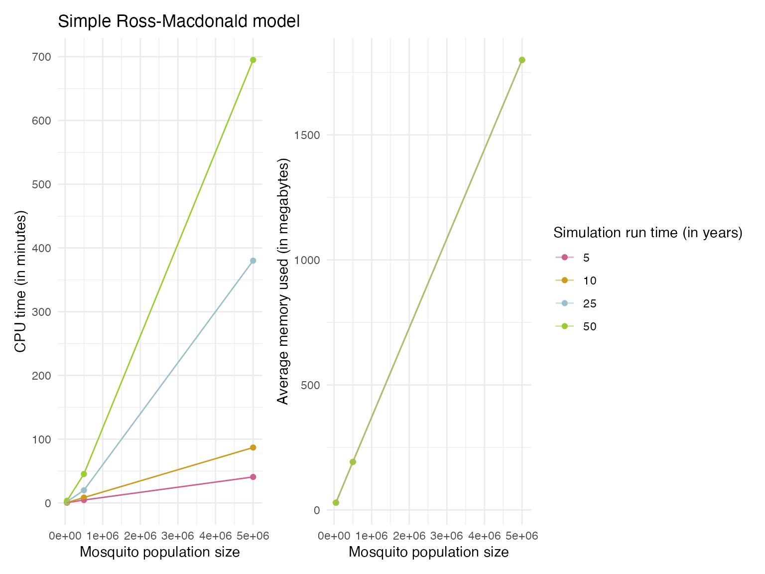
Figure 3. The profiling results showing the CPU times and memory usage for simulation runs with varying mosquito population sizes
Conclusions
Although SLiM is a powerful forward genetic simulation tools with
extensive potential applications, unfortunately it does not seem
appropriate for our use-case. The main appeal for integration with the
SIMPLEGEN pipeline was the ability to use tree-sequence recording,
however, this functionality is not available in the multi-species model
that we would require for our simulations. In addition, given SLiM was
developed with other genetic applications in mind, it is not
computationally efficient for epidemiological models such as a
vector-host model. Future considerations for SIMPLEGEN will be to
integrate conversion of the transmission record into a
tskit-appropriate .tree structure for more
efficient storage and downstream use of msprime and
tskit functionalities such as genetic statistic
calculations.
Some notable and useful resources/papers
Below is a list of some useful papers citing SLiM as well as other useful resources.
Champer et al (Champer et al. 2022) use SLiM for simulations of Anopheles mosquito gene drive. Their SLIM models are available on GitHub (useful to look at): https://github.com/jchamper/ChamperLab/blob/main/Mosquito-Drive-Modeling/
(Matthey-Doret 2021) describes R wrapper {
SimBit} that implements tree structures for output (might be useful to see how tskit is implemented in another C++/R framework)(Cury et al. 2022) useful guide on how to build appropriate bacterial models in SLiM, and with a good overview of implemented models in SLiM with rationale for model parameters and coding choices etc. They use nonWF SLiM model with tree-sequence recording + recapitation in
msprime, first run forward simulation and then use recapitation on ancestral branches to produce coalescence.(Cao et al. 2021) useful guide on how to build haploid simulations in SLiM
(Hardy 2022) simulates subpopulations (ie. demes) usng SLiM to model individual genomes, which can reproduce, mutate, recombine and die
(Sabin et al. 2022) use SLiM to model Mycobacterium based on nucleotide sequences, SLiM model parameters available on github, eg: https://github.com/sjsabin/mcan_popgen/blob/main/simulations/base/base.slim
{stdpopsim}((Adrion et al. 2020)) catalog of different species and demographic history (include Anopheles as per Miles 2017 params)-
{slimr}R package (Dinnage et al. 2021) that interfaces with SLiM 3.0: https://github.com/rdinnager/slimr/Downside: seems like its not compatible with SLiM 4.0
Workshop recording: https://zoom.us/rec/share/T5thlw67U8T3-BNQUJoZiaKTCSk2xeQTkyDpvOwvtUnPRO7VCE8tvJzUJsGTYnkd.xHFECYM5vDtJdp12 (passcode: uk5^G$z7)
Workshop code: https://github.com/rdinnager/slimr_workshop_CBA
-
fwddpp(C++ template library) (Thornton 2014) orders of magnitude faster than SLiMuse cases: large Ns and selection
fastest algorithm
nonstandard fitness models and/or modeling fitness-to-fitness relationships
maximize runtime efficiency for particular demo scenario
unsure if can handle haploids
-
Some useful examples of how others have used SLiM and documented their workflows are below:
(Blischak, Barker, and Gutenkunst 2020) exported individual genotype data from each simulation as vcfs (
.outputVCFSample()). They also have publicly available code for their SLiM models implemented in python (https://github.com/pblischak/inbreeding-sfs/tree/master/sims/SLiM)(E. C. Anderson 2021) provides useful a description of SLiM as part of larger pipeline (the SLiM output can be used downstream using R package {
CKMRpop}). Note: the output described here seems very similar to the transmission record of IDs produced by SIMPLEGEN.