Designing a study

This tutorial demonstrates how you can use the DRpower package in the design phase of a pfhrp2/3 deletion study to ensure you have adequate power. This takes a purely statistical view of the problem; the results presented here should be taken alongside other considerations such as logistical, financial and ethical factors.

This tutorial covers:

Using sample size tables
Interpreting power curves
Refining sample sizes based on real-world constraints and recalculating power
Accounting for dropout, and working out how many suspected cases to enrol
Using the same study design for other molecular end-points, including detecting rare variants and estimating a drug resistance marker to within a known margin of error

1. Consult sample size tables

Our aim is to conduct a multi-site survey to test the prevalence of pfhrp2/3 deletions against a defined threshold. The question is; how many sites should I use and how many samples per site?

The fastest way to get an idea of adequate sample size is to consult pre-computed sample size tables. These are distributed as part of the DRpower package and can be accessed through the df_ss object. This data.frame contains sample sizes for a wide range of parameter combinations, so we will start by filtering down to the parameters we care about. In our case, we will power the study to detect a prevalence of 10% deletions in our domain, and we will assume an intra-cluster correlation coefficient of 0.05 based on historical data:

# get sample size table for parameters of interest
get_sample_size_table(prevalence = 0.1, ICC = 0.05, prev_thresh = 0.05)
#> # A tibble: 19 × 2
#>    n_clust `0.1`
#>      <int> <dbl>
#>  1       2    NA
#>  2       3    NA
#>  3       4    NA
#>  4       5   496
#>  5       6   113
#>  6       7    68
#>  7       8    51
#>  8       9    37
#>  9      10    30
#> 10      11    25
#> 11      12    22
#> 12      13    17
#> 13      14    15
#> 14      15    14
#> 15      16    13
#> 16      17    11
#> 17      18    11
#> 18      19    10
#> 19      20     9

Note that these values are only valid if you intend to analyse your data using the DRpower model. If you plan to do a different statistical analysis then you need a different power analysis.

We can see that at least 5 sites are needed, otherwise sample sizes are too large to be reported in this table. It’s also interesting to note that the total sample size (n_clust * N_opt) decreases as we recruit more sites For example, a 6-site design would require 678 samples in total, but a 10-site design would require only 300. This is one of many arguments for recruiting as many sites as possible.

Let’s assume that we can only recruit 6 sites for logistical reasons, meaning we are aiming for 113 samples per site. These sites can be chosen through randomisation of all health facilities, or by using predesignated sentinel surveillance sites. In the latter case, it is important that sentinel sites are chosen to be representative of the population in the domain as a whole (e.g. in terms of demographic and social characteristics), otherwise we risk getting a biased view of the prevalence of pfhrp2/3 deletions.

2. Consult power curves

Although sample size tables are a good starting point, they do not tell us how power is changing with \(N\). It could be that the curve is very steep, in which case dropping even just a few samples would really hurt our power. On the other hand, it could be that the curve is very shallow, in which case we have some more wiggle room.

All of the power curves that were used to produce the sample size tables are distributed with the DRpower package and accessible via the df_sim object. We can also visualise them directly using the plot_power() function:

# plot power as a function of per-site sample size
plot_power(n_clust = 6, prevalence = 0.1, N_max = 200)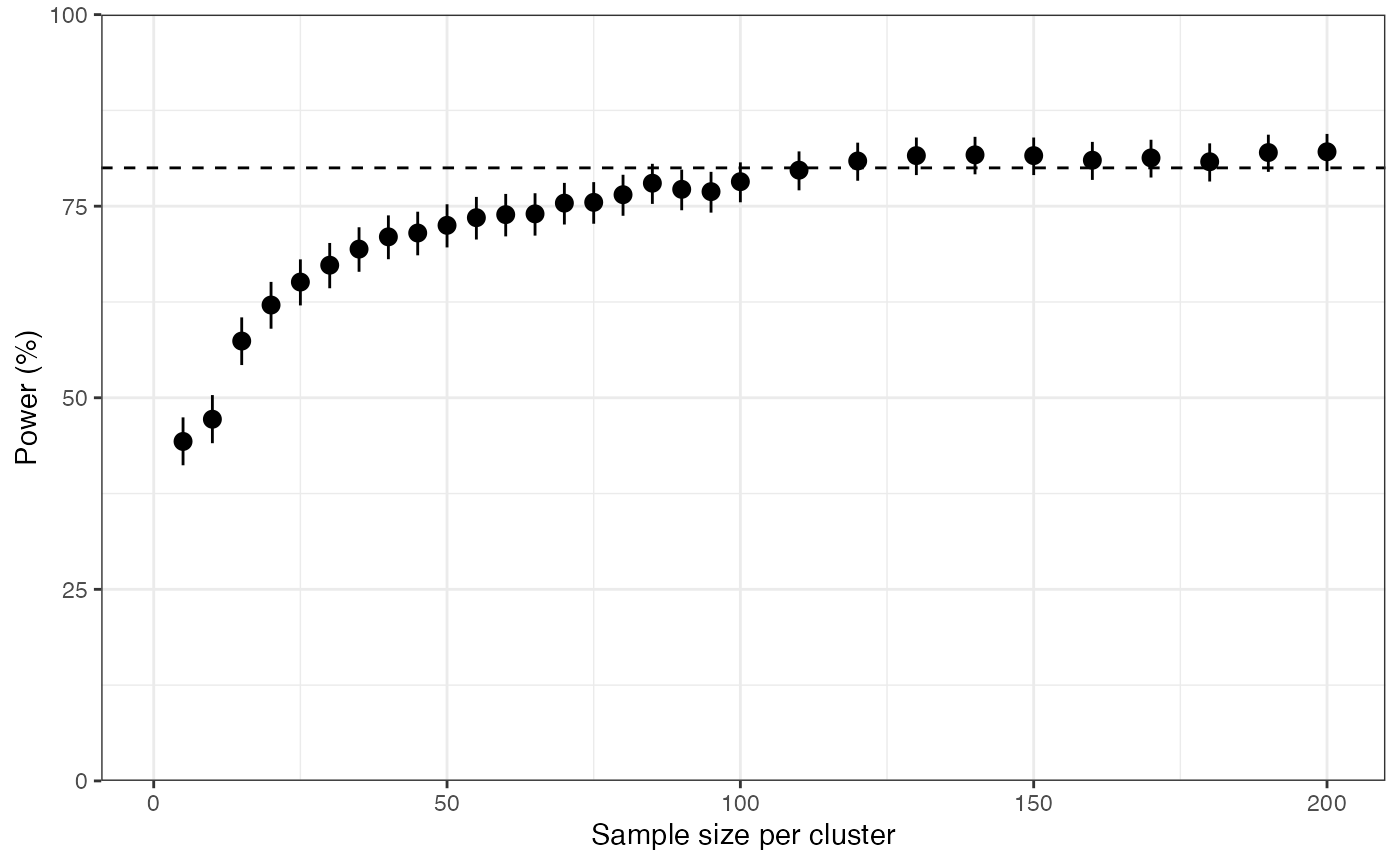

We find that the power curve is fairly shallow around the chosen value of N = 113. For example, the value N = 70 still achieves 75% power. We need to be pragmatic about these numbers, and not stick dogmatically to the target value of 80% power without thinking about what it means. We should remember that power is defined as the probability of finding an interesting result if it is there, so a study with 75% power has almost as good a chance of success as a study with 80% power. It is certainly not the case that if we fail to hit 80% then the study is completely invalid. This is important because a drop in sample size from 113 per site to 70 per site may be the difference between a study that is feasible to conduct and one that is not. We need to balance these factors against each other when coming up with a study design.

That being said, we should not allow power to drop too low or the study may not be worth doing. In our case we will stick to the target value of 113 samples per site, as we believe we can raise funds to this level and successfully carry out the study with this sample size.

3. Refine sample sizes

Next, we should examine our 6 sites individually to see if they are able to recruit 113 samples. Ideally, this should be informed by historical incidence trends at each of the sites, which can give a good indication of how many malaria cases tend to be seen throughout the transmission season.

In our case, let’s assume that two sites are in low transmission areas, meaning they can only recruit 60 samples during the study time frame. Another two sites are very small, and only have the capacity to enrol 40 samples due to staffing issues.

The question is - how badly do these smaller sample sizes hurt our power? We cannot work this out from sample size tables or power curves because these assume the same sample size in each site. But we can explore power directly using the get_power_threshold() function:

get_power_threshold(N = c(113, 113, 60, 60, 40, 40),   # new sample sizes per site
                    prevalence = 0.1,
                    ICC = 0.05,
                    prev_thresh = 0.05,
                    reps = 1e3)
#>   prev_thresh power lower upper
#> 1        0.05  73.7 70.85 76.41

We find that power is slightly lower than before, probably around 74%. We could try to balance things out by obtaining more samples from our remaining two sites:

get_power_threshold(N = c(250, 250, 60, 60, 40, 40),   # rebalanced cluster sizes
                    prevalence = 0.1,
                    ICC = 0.05,
                    prev_thresh = 0.05,
                    reps = 1e3)
#>   prev_thresh power lower upper
#> 1        0.05  77.7 74.99 80.25

This rebalancing has helped, power is now back up to around 78%, but it comes at the cost of obtaining more samples. The total sample size has now gone up to 700 from the original 678.

As an aside, compare this with what happens if we were able to recruit just one more site, rather than expanding our existing sites:

get_power_threshold(N = c(113, 113, 60, 60, 40, 40, 40),   # one more site of size 40
                    prevalence = 0.1,
                    ICC = 0.05,
                    prev_thresh = 0.05,
                    reps = 1e3)
#>   prev_thresh power lower upper
#> 1        0.05  78.2 75.51 80.72

Power is now recovered to around 78% while the total sample size is only 466. This emphasises the point that where possible we should put our efforts into recruiting more sites rather than increasing per-site sample sizes.

In our case, we assume a hard limit of 6 sites, so we will stick with the rebalanced numbers:

# final sample sizes per site
N <- c(250, 250, 60, 60, 40, 40)

This should give us power of around 78% (somewhere in the range 75% to 80%), which is a balance between the target power we would like and what we can realistically achieve given real world constraints.

4. Account for dropout

It is always sensible to account for dropout, meaning samples that, for whatever reason, do not make it all the way to the final analysis. Reasons can include people withdrawing consent from the study, RDTs getting lost, samples getting contaminated or failing the molecular laboratory methods. Although these events might be unlikely, failing to account for potential dropout makes our study quite fragile to unforeseen events that can hurt our power. A local technician is often the best person to give informed advice on the expected dropout. In our case we will assume dropout of 10%, meaning we need to divide through by 0.9:

N_adjusted <- ceiling(N / 0.9)

print(N_adjusted)
#> [1] 278 278  67  67  45  45

The ceiling() function rounds values up to the nearest whole number.

Note that these numbers refer to confirmed malaria cases (by some gold standard that is not HRP2-based RDTs). When designing a study we may need to know how many suspected malaria cases to enrol, which may be much higher as suspected malaria cases often come back negative due to the symptoms overlapping with other illnesses. To calculate the number of suspected cases that we need to enrol we should divide our sample sizes through by the expected positive fraction. For example, if we expect 40% of suspected cases to come back positive then we would do the following:

N_suspected <- ceiling(N_adjusted / 0.4)

print(N_suspected)
#> [1] 695 695 168 168 113 113

Here, we have assumed the same positive fraction over all sites, but if you have data from individual sites that can be used then that is even better. We might also expect the positive fraction to have a relationship with transmission intensity, in which case we can incorporate this information.

To be completely clear about what each of these numbers mean:

N_suspected gives the number of suspected malaria cases that we expect to enrol (1952 in total)
N_adjusted gives the number of confirmed malaria cases that we expect to enrol (780 in total)
N gives the number of confirmed malaria cases that we expect to end up with at the end of the study after dropout (700 in total)

At this stage, it is worth doing a sanity check with the staff at the local facilities to ensure they will be able to enrol these numbers within the study period. This is also the point at which we can do full budget calculations.

5. Iterate and improve

Although we have completed a full statistical analysis of the number of sites and samples, we should not think of these values as set in stone. Rather, they give a first sketch of a study design that may be workable, and that has good statistical properties. But if this turns out to be impractical, either from logistical or budgetary perspectives, then we are free to explore variations until we find something that will work. What we should not do is 1) continue doggedly with a plan that we believe will fail in practice, or 2) throw all statistical arguments out the window and just collect whatever samples we can get our hands on. It is usually possible to balance statistical arguments against real world constraints to get something that satisfies both.

6. Detecting rare variants (bonus section)

We often plan on using the same samples for multiple reasons. For example, it is common to look for drug resistance markers at the same time as pfhrp2/3 deletions. In this case, we should perform a separate power analysis and sample size calculation for these other end-points and always take the largest sample size between the two analyses, as this is the one that will give sufficient power over all end-points.

The DRpower package contains simple functions for exploring other questions. For example, imagine we are looking to detect the presence of rare variants, such as pfk13 mutations conferring partial resistance to artemisinin. Here, we are asking whether the prevalence is greater than zero in the domain, and a single positive result confirms that there are. The function get_power_presence() tells us our power to detect any mutants. Similar to the pfhrp2/3 deletion analysis, this assumes we will run a multi-site study and summarise results over all sites, meaning we need to account for intra-cluster correlation:

# get power to detect a 1% variant at the domain level
get_power_presence(N = N, prevalence = 0.01, ICC = 0.05)
#> [1] 86.5711

We can see that the same sample sizes from the pfhrp2/3 deletion study design also give us more than 80% power to detect rare variants at the domain level. Another way to approach this problem is to use the function get_sample_size_presence(), which tells us how many samples we need in each site to achieve 80% power:

# how many samples would we need to achieve 80% power in the presence analysis
get_sample_size_presence(n_clust = 6, prevalence = 0.01, ICC = 0.05)
#> [1] 58

So six sites with 58 samples each would do it. From our pfhrp2/3 analysis we have variable sample sizes, some above this level and some below, which is why the get_power_presence() method was useful.

What if we are not interested in summarising at the domain level, and instead we want to know our power in each of the individual sites? We can use the same functions as before, now run independently over each of the sites. We should fix the ICC at zero because this is no longer a multi-site study:

# how many samples are needed in an independent analysis
get_sample_size_presence(n_clust = 1, prevalence = 0.01, ICC = 0)
#> [1] 161

# get power to detect a 1% variant in each of the individual sites
mapply(get_power_presence, N, MoreArgs = list(ICC = 0))
#> [1] 91.89415 91.89415 45.28434 45.28434 33.10282 33.10282

We find that 161 samples are needed for a single site to be powered to detect a rare variant at 1% prevalence. Accordingly, only our large sites (250 samples) achieve power over 80%, and the smaller sites with 60 and 40 samples have power below 50%. Therefore we would conclude that 4 out of our 6 sites are underpowered at the individual level, and so we may be better off pooling results to the domain level.

7. Controling the margin of error (bonus section)

What if we also plan on using the same samples to look for a drug resistance marker that we already believe to be at high prevalence? In this case, it can be useful to consider what will be the expected margin of error in our analysis. This is not the same as a power analysis, as we are not conducting a hypothesis test. Rather, we are trying to choose a sample size that gives us a certain level of precision.

The get_sample_size_margin() function tells us the per-site sample size needed to achieve a given margin of error (MOE) if we plan on pooling results over multiple sites. Here, we assume that the prevalence of the marker is 20% in the population, and we aim to estimate this to within plus or minus 10%:

# get sample size needed to achieve 10% MOE if prevalence is 20% and we have 6 sites
get_sample_size_margin(MOE = 0.1, n_clust = 6, prevalence = 0.2, ICC = 0.05)
#> [1] 20

We only need 20 samples to achieve this level of precision, which we are well above. We can also use the get_margin() function to tell us what our MOE would be given a known sample size:

# get MOE assuming 40 samples in each of 6 sites
get_margin(N = 40, n_clust = 6, prevalence = 0.2, ICC = 0.05)
#>    lower    upper 
#> 11.30813 28.69187

With 40 samples we would expect our 95% CI to range from around 11.3% to 28.7%, in other words a MOE of around 8.7%.

The formula used above is extremely simple. It does not allow for different sample sizes per site, and it also assumes that we know the ICC exactly rather than estimating it from data. An alternative approach is to use the DRpower Bayesian model to estimate the prevalence. In other words, we plan on using the get_prevalence() function to obtain a 95% Bayesian credible interval (CrI). If we plan to estimate prevalence this way, then we should use the function get_margin_Bayesian() to estimate our MOE. This function works by simulation, and allows for different sample sizes in each site:

# get MOE when using DRpower Bayesian model
get_margin_Bayesian(N, prevalence = 0.2, ICC = 0.05)
#>       estimate   CI_2.5  CI_97.5
#> lower  12.6323 12.03405 13.23055
#> upper  31.0595 30.12544 31.99356

Using this method, we expect our 95% CrI to range from around 12.6% to 31%. Note that this MOE is different in the lower and upper directions meaning the CrI is not symmetric. It is also narrower at the lower end than our previous get_margin() estimate, but wider at the upper end. The Bayesian model makes different assumptions, and so in general we shouldn’t expect the CrI to be the same as the CI.

In summary…

We have sample sizes (N) that we are happy with for our pfhrp2/3 analysis. These don’t quite achieve 80% power, but they are not far off. They have been chosen taking into account logistical and feasibility constraints as well as statistical considerations. We also know the number of suspected malaria cases that we need to enrol (N_suspected).
The same sample sizes give us 86% power to detect rare pfk13 variants at 1% in the population when summarised at the domain level. We do not have power to detect rare variants at the individual site level in most sites.
The same sample sizes give us a margin of error of around 10% when estimating the prevalence of a variant at 20% in the population.

Notice that this summary considers all end-points for the same sample sizes. We have now arrived at a detailed plan and have a good idea of what we can expect from our results. It is up to us to decide if we want to go ahead with this plan, or if we want to revisit assumptions and modify the plan accordingly.

Bob Verity