Power and Sample Size in the DRpower Model
Bob Verity
Last updated: 08 Nov 2024
Source:vignettes/rationale8_power.Rmd
rationale8_power.Rmd8. Estimating power via simulation
The power of a hypothesis test is intrinsically linked to the method we plan to use in our statistical analysis. We have found that if we plan to conduct a z-test on our data then, for the parameter values described in the 2020 Master Protocol, we will need 1126 samples. But what if we change our analysis plan to the Bayesian model in DRpower? Can we calculate power under this new approach?
The answer is both yes and no. We cannot produce a neat formula for the power as we could for the z-test as this Bayesian model is simply too involved. We can, however, estimate the power by simulation. We can follow these steps:
- Choose true values of parameters like the prevalence (\(p\)) and the intra-cluster correlation (\(r\)). These values represent the alternative hypothesis that we are interested in. This is similar to assuming a prevalence value of 8% or 3.2% in the Master Protocol.
- For a particular number of sites (\(c\)) and sample size per site (\(n\)), simulate data from the beta-binomial model. Analyse this simulated data using the DRpower method, and establish whether we conclude that prevalence is above 5% or not.
- Repeat this simulation-analysis step many times (hundreds or thousands). Count the proportion of times that we come to the correct conclusion. This proportion is our estimate of the empirical power.
One major advantage of the empirical power method is that it uses the exact analysis approach that we will use on our real data, meaning there are no approximations or fudging over uncertainty. The main downsides of this approach are; 1) it is based on a random sample, meaning power is only estimated and not calculated exactly, 2) it can take a long time to estimate if the analysis step is slow. These issues are mitigated to some extent in DRpower by pre-computing power for a wide range of parameter values. The results are made available with the DRpower package, one such set of results is shown below:
# calculate power by z-test for same parameters
df_ztest <- data.frame(n = 5:200) %>%
  mutate(n_clust = 6,
         N = n*n_clust,
         p = 0.1,
         mu = 0.05,
         ICC = 0.05,
         Deff = 1 + (n - 1)*ICC,
         power = pnorm(abs(p - mu) / sqrt(Deff * p*(1 - p) / N) - qnorm(1 - 0.05/2)))

plot_power(n_clust = 6, prevalence = 0.1, ICC = 0.05, prev_thresh = 0.05, N_max = 200) +
  geom_line(aes(x = n, y = 1e2*power, colour = "z-test"), data = df_ztest) +
  ggtitle("Assumptions:\nclusters = 6, prevalence = 10%, ICC = 0.05")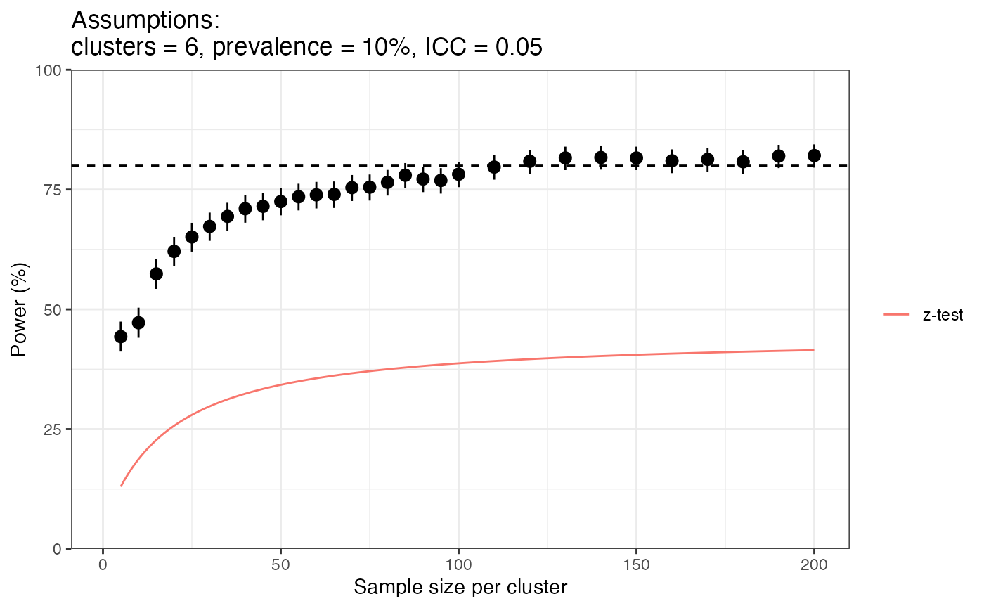
There is some random noise in this plot, but the overall trend is clear. Power increases quickly at first and then plateaus out for larger sample sizes. Power reaches 80% for the DRpower method at around 113 samples per site In contrast, the z-test method never reaches the 80% power level, and in fact would never make it over 50% even for an infinitely large sample size.
Why does the DRpower model have so much higher power than the z-test? This is not straightforward to answer, as the two approaches come from completely different statistical philosophies, but one very important difference is in the specific hypotheses that we are testing. In the z-test approach we are trying to disprove a single hypothesis; that the prevalence is exactly equal to the threshold. On the other hand, in the Bayesian approach we are comparing two hypotheses; 1) the prevalence is above the threshold, vs. 2) the prevalence is below the threshold. By “below the threshold” we don’t mean exactly on the threshold, but rather anywhere below it. This is sometimes referred to as a composite hypothesis test because we are assuming a range of values rather than a single value. This composite hypothesis is easier to disprove because we are being less pessimistic about the prevalence of pfhrp2/3 deletions. So, this boils down to a difference in assumptions under the null hypothesis. We feel that the Bayesian perspective is justified here because a “low” prevalence of pfhrp2/3 deletions will often mean values below the threshold rather than exactly on it.
8.1. Sample size calculation
Once we have a power curve like the one above, we can work out what sample size we would need to achieve any given power. For the simulation-based approach this will only be approximate because of noise in the power curve. We take a three-step approach:
- Use linear interpolation between a fixed set of simulations (i.e., join the dots in the plot above). Find the first value of the sample size for which the power exceeds 80%.
- Intuitively, we would expect per-site sample sizes to decrease as the number of sites increases. In some rare cases this method can give the opposite result due to random fluctuations. We remove this effect by manually modifying results so that sample size can never decrease with more sites.
- Sample sizes greater than 2000 are coded as
NAbecause these are prohibitively large. Sample sizes less than 5 are fixed at 5 because it would not be worth enrolling a site and collecting fewer than this many samples.
For an assumed ICC of 0.05 based on historical data, this leads to the sample size table shown below:
| n_clust | 8 | 9 | 10 | 11 | 12 | 13 | 14 | 15 | 16 | 17 | 18 | 19 | 20 |
|---|---|---|---|---|---|---|---|---|---|---|---|---|---|
| 2 | NA | NA | NA | NA | NA | 344 | 140 | 62 | 38 | 33 | 22 | 18 | 14 |
| 3 | NA | NA | NA | NA | 172 | 69 | 41 | 26 | 20 | 16 | 14 | 12 | 9 |
| 4 | NA | NA | NA | 128 | 60 | 33 | 22 | 16 | 13 | 10 | 9 | 8 | 7 |
| 5 | NA | NA | 496 | 75 | 36 | 22 | 16 | 10 | 7 | 7 | 5 | 5 | 5 |
| 6 | NA | NA | 113 | 47 | 25 | 16 | 12 | 9 | 6 | 5 | 5 | 5 | 5 |
| 7 | NA | NA | 68 | 30 | 18 | 13 | 10 | 7 | 6 | 5 | 5 | 5 | 5 |
| 8 | NA | 416 | 51 | 23 | 15 | 10 | 9 | 7 | 5 | 5 | 5 | 5 | 5 |
| 9 | NA | 138 | 37 | 20 | 13 | 10 | 8 | 6 | 5 | 5 | 5 | 5 | 5 |
| 10 | NA | 85 | 30 | 15 | 12 | 8 | 6 | 5 | 5 | 5 | 5 | 5 | 5 |
| 11 | NA | 66 | 25 | 13 | 10 | 8 | 6 | 5 | 5 | 5 | 5 | 5 | 5 |
| 12 | NA | 45 | 22 | 12 | 9 | 7 | 5 | 5 | 5 | 5 | 5 | 5 | 5 |
| 13 | NA | 40 | 17 | 11 | 8 | 5 | 5 | 5 | 5 | 5 | 5 | 5 | 5 |
| 14 | 438 | 34 | 15 | 10 | 7 | 5 | 5 | 5 | 5 | 5 | 5 | 5 | 5 |
| 15 | 179 | 29 | 14 | 9 | 7 | 5 | 5 | 5 | 5 | 5 | 5 | 5 | 5 |
| 16 | 122 | 28 | 13 | 8 | 5 | 5 | 5 | 5 | 5 | 5 | 5 | 5 | 5 |
| 17 | 122 | 22 | 11 | 8 | 5 | 5 | 5 | 5 | 5 | 5 | 5 | 5 | 5 |
| 18 | 84 | 21 | 11 | 7 | 5 | 5 | 5 | 5 | 5 | 5 | 5 | 5 | 5 |
| 19 | 70 | 19 | 10 | 7 | 5 | 5 | 5 | 5 | 5 | 5 | 5 | 5 | 5 |
| 20 | 67 | 18 | 9 | 6 | 5 | 5 | 5 | 5 | 5 | 5 | 5 | 5 | 5 |
For example, if we assume the prevalence of pfhrp2/3 deletions is 10% in the population, and we will survey 10 sites, then we need a sample size of 30 per site (300 total).
Compare this with the sample size table we would get if we were using the z-test:
| n_clust | 8 | 9 | 10 | 11 | 12 | 13 | 14 | 15 | 16 | 17 | 18 | 19 | 20 |
|---|---|---|---|---|---|---|---|---|---|---|---|---|---|
| 2 | NA | NA | NA | NA | NA | NA | NA | NA | NA | NA | NA | NA | NA |
| 3 | NA | NA | NA | NA | NA | NA | NA | NA | NA | NA | NA | NA | 254 |
| 4 | NA | NA | NA | NA | NA | NA | NA | NA | NA | 473 | 114 | 64 | 44 |
| 5 | NA | NA | NA | NA | NA | NA | NA | NA | 130 | 64 | 42 | 31 | 25 |
| 6 | NA | NA | NA | NA | NA | NA | 666 | 96 | 51 | 34 | 26 | 21 | 17 |
| 7 | NA | NA | NA | NA | NA | NA | 96 | 48 | 32 | 24 | 19 | 15 | 13 |
| 8 | NA | NA | NA | NA | NA | 124 | 52 | 32 | 23 | 18 | 15 | 12 | 11 |
| 9 | NA | NA | NA | NA | 297 | 64 | 36 | 24 | 18 | 15 | 12 | 10 | 9 |
| 10 | NA | NA | NA | NA | 105 | 43 | 27 | 20 | 15 | 12 | 10 | 9 | 8 |
| 11 | NA | NA | NA | 619 | 64 | 33 | 22 | 16 | 13 | 11 | 9 | 8 | 7 |
| 12 | NA | NA | NA | 153 | 46 | 27 | 18 | 14 | 11 | 9 | 8 | 7 | 6 |
| 13 | NA | NA | NA | 88 | 36 | 22 | 16 | 12 | 10 | 8 | 7 | 6 | 6 |
| 14 | NA | NA | NA | 61 | 29 | 19 | 14 | 11 | 9 | 8 | 7 | 6 | 5 |
| 15 | NA | NA | 308 | 47 | 25 | 17 | 13 | 10 | 8 | 7 | 6 | 5 | 5 |
| 16 | NA | NA | 144 | 39 | 22 | 15 | 11 | 9 | 8 | 7 | 6 | 5 | 5 |
| 17 | NA | NA | 94 | 33 | 19 | 14 | 10 | 8 | 7 | 6 | 5 | 5 | 5 |
| 18 | NA | NA | 70 | 28 | 17 | 12 | 10 | 8 | 7 | 6 | 5 | 5 | 5 |
| 19 | NA | NA | 56 | 25 | 16 | 11 | 9 | 7 | 6 | 5 | 5 | 5 | 5 |
| 20 | NA | NA | 46 | 22 | 14 | 11 | 8 | 7 | 6 | 5 | 5 | 5 | 5 |
For the same assumption of 10% prevalence we would need 15 sites of 308 individuals (4620 total)!
8.2. How to choose final sample sizes
Using the DRpower table above (not the z-test table!) we can come up with reasonable values for the sample size per site. But these values assume the same sample size per site, which is often not true in practice. At this point, we need to switch away from simple tables and perform a power analysis that is more bespoke to our problem. The steps are roughly as follows:
- Work out how many clusters are feasible within a given province based on logistical and budgetary considerations.
- Work out what prevalence of pfhrp2/3 deletions you want to power your study for. A value of 10% is a reasonable default to use here.
- Use these values to look up the corresponding minimum sample size from the table above. This is your first rough estimate of sample size per cluster.
- Buffer these values for potential dropout. Also note that this table gives the number of confirmed malaria positive individuals, but you may want to design the study based on the total number tested, which may be considerably higher. For example, if you suspect that 40% of suspected malaria cases end up being confirmed then you would need to divide your sample size by 0.4.
- Examine whether it will be possible to recruit this many samples in each of your sites. This may depend on things like catchment population size, staff numbers, and malaria transmission intensity throughout the season. It may be that in some cases it is not possible to reach these numbers.
- For your newly refined sample size estimates, estimate power
directly using the
get_power_threshold()function.
The design tutorial goes through all of these steps in detail.