The nugget and the dispersion: two views of one noise

Two noise quantities appear in the walkthrough: the nugget ratio $\eta$, estimated while fitting the kernel hyperparameters, and the Negative-Binomial dispersion $r$, used when the prediction interval is assembled. A natural worry is that the same observation noise is being modelled twice. This short note explains how the two relate: they describe the same physical fact — counts scatter around their underlying rate — but on different scales, with different shapes, and doing different jobs.

Two jobs on two scales

	nugget ratio $\eta$	dispersion $r$
scale	log (the field $g$)	natural counts
noise shape	Gaussian, one variance for every cell	Negative-Binomial, variance $\lambda + \lambda^2/r$
stage	fitting and smoothing	the prediction interval only
what it does	stops the kernels explaining noise with smoothness; tells the smoother how much to de-weight each observed week	adds the spread of a future count around its rate
what it moves	the hyperparameters, the predicted rate, and the rate-uncertainty part of the interval	the interval width only

The nugget is the count scatter as the fitting stage sees it: everything happens on the standardised $\log(1+y)$ scale, where the scatter is approximated as Gaussian with a single homoscedastic variance. The dispersion is the count scatter as it really is: heteroscedastic on the natural scale, growing with the rate.

Why it is not double counting

The prediction interval is built from the law of total variance,

$$\operatorname{Var}[y] = \underbrace{\mathbb{E}\!\big[\lambda + \tfrac{\lambda^2}{r}\big]}_{\text{count noise}} + \underbrace{\operatorname{Var}[\lambda]}_{\text{rate uncertainty}} ,$$

and the two quantities feed different terms. Noisy observations limit how well the rate $\lambda$ can be known — that is the nugget’s contribution, flowing through the GP posterior into $\operatorname{Var}[\lambda]$. A future count then scatters around $\lambda$ even if it were known exactly — that is the dispersion’s contribution, the first term. One quantity is about learning the rate from noisy data; the other is about a new count being noisy. Both derive from the same source, but each appears exactly once.

The quantitative link

The two are not independent descriptions either. By the delta method, a Negative-Binomial count viewed on the log scale has approximate variance

$$\operatorname{Var}[\log y] \;\approx\; \frac{1}{\lambda} + \frac{1}{r},$$

which flattens towards the constant $1/r$ once counts are moderately large:

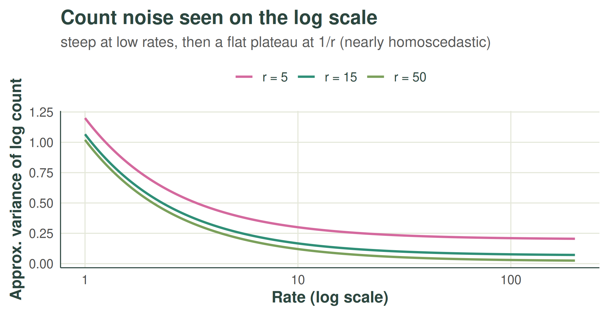
That plateau is exactly why a single homoscedastic log-scale nugget is a reasonable stand-in for heteroscedastic count noise during fitting: over the bulk of the data the log-scale noise level barely varies, and the fitted $\eta$ lands near its average. So the nugget can loosely be read as the log-scale image of the Negative-Binomial noise — plus any slack from the $\log(1+y)$ transformation itself.

The approximation frays where the curve is steep: at very low rates the $1/\lambda$ term dominates and changes from cell to cell, so sparse sites are noisier on the log scale than the single nugget admits. This is the same low-count territory flagged in the walkthrough’s caveats — the two warnings are one phenomenon.