The Kronecker trick: why weave is fast

A weave model has one cell per site and week: $N = n \cdot n_t$ cells in total. The Gaussian-process covariance over those cells is an $N \times N$ matrix — at 1000 sites and five years of weeks that is around 67 billion entries. weave never forms it, never inverts it, and never approximates it. Everything in the walkthrough — fitting the hyperparameters and computing the exact part of the prediction interval — stays exact because the covariance is separable, and separable covariances can be handled through their small factors alone. This article explains the two identities that make that work.

One small matrix per dimension

The model assumes the covariance factorises into a spatial part and a temporal part:

$$K \;=\; K_{\text{space}} \otimes K_{\text{time}},$$

where $K_{\text{space}}$ is $n \times n$, $K_{\text{time}}$ is $n_t \times n_t$, and $\otimes$ is the Kronecker product — a recipe that builds the one enormous matrix from the two small ones: the covariance between cell $(s, t)$ and cell $(s', t')$ is simply $K_{\text{space}}[s, s'] \times K_{\text{time}}[t, t']$.

Seeing the structure

A toy problem makes the recipe concrete: 3 sites × 8 weeks, so 24 cells and a 24 × 24 covariance. We build it from the two small pieces.

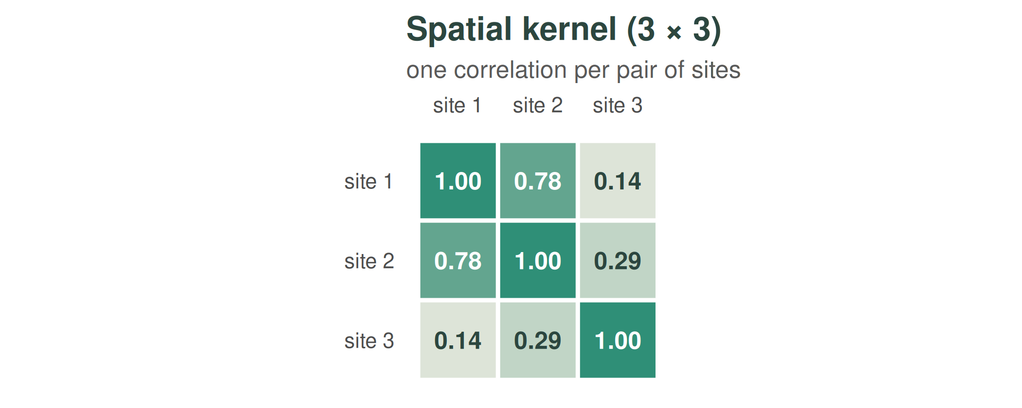
The spatial kernel holds one correlation per pair of sites. In the toy, sites 1 and 2 sit close together and site 3 sits far away — and the matrix says exactly that:

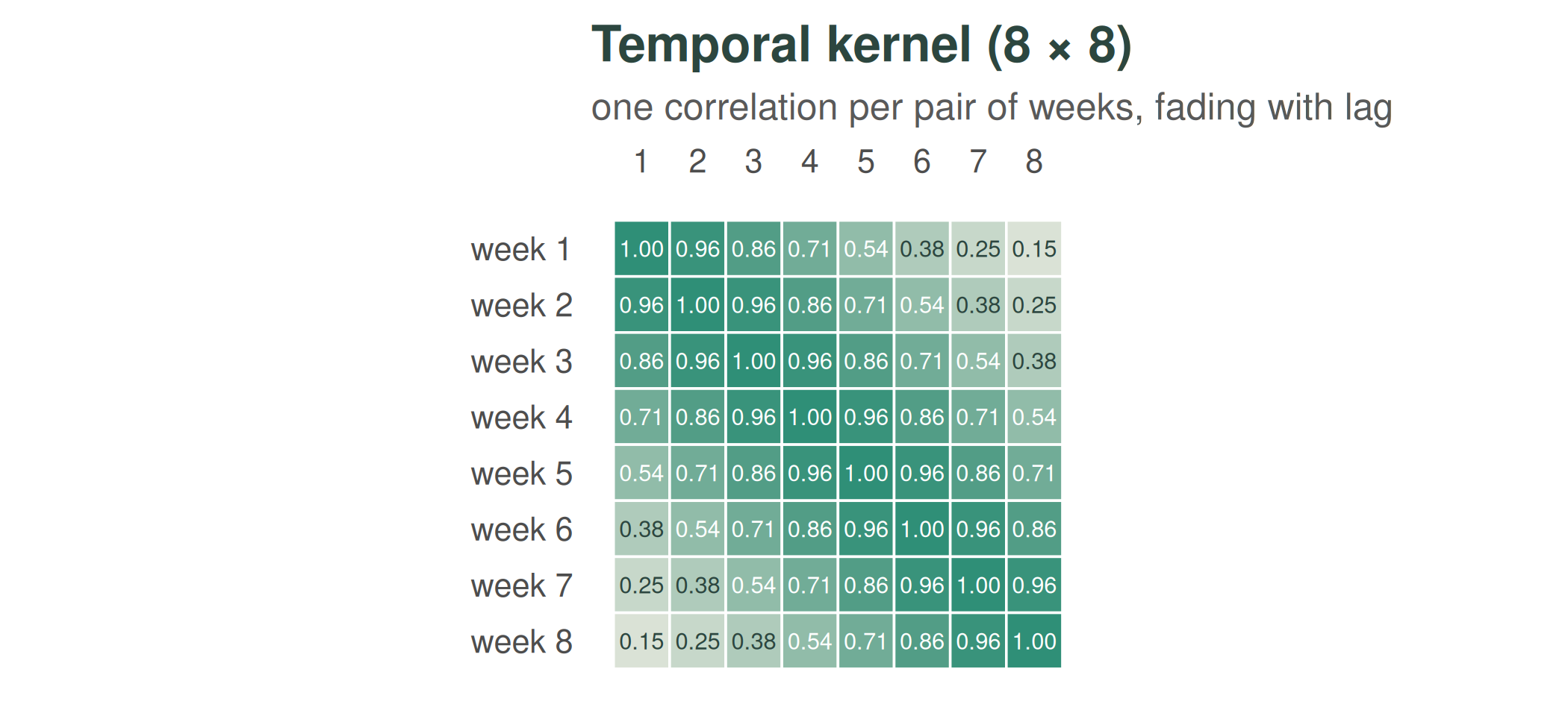
The temporal kernel holds one correlation per pair of weeks. Its banded shape says that nearby weeks look alike and the resemblance fades with lag:

The Kronecker product assembles the full covariance from those two. Lay out a 3 × 3 grid of blocks — one block per pair of sites — and make each block a copy of the whole 8 × 8 temporal kernel, dimmed by that site pair’s spatial correlation. Sites 1 and 2 are highly correlated (0.78), so their off-diagonal blocks are nearly as strong as the diagonal; site 3 is far from site 1 (0.14), so their block — outlined in deep green below — is the same temporal pattern, just faint:

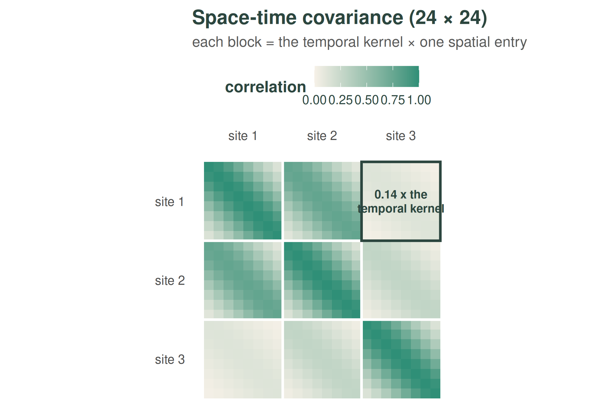
Read any single entry the same way: the covariance between cell $(s, t)$ and cell $(s', t')$ is $K_{\text{space}}[s, s'] \times K_{\text{time}}[t, t']$ — always a product of one number from each small matrix. That is all $\otimes$ means, and it is why the 24 × 24 matrix (or the 67-billion-entry one) never needs to exist: the two small matrices carry every entry implicitly.

Statistically, separability says the shape of the temporal correlation is the same at every site (and vice versa) — a modelling assumption, and the price of everything below.

Identity 1: determinants and quadratic forms (used in fitting)

Fitting the hyperparameters requires the log marginal likelihood of the plug-in field $g$, which needs $\log|K|$ and $g^\top K^{-1} g$ — normally hopeless at size $N$. Because the covariance is a Kronecker product plus a diagonal nugget, eigendecomposing the small factors $R_{\text{space}} = U_s \Lambda_s U_s^\top$ (size $n$) and $R_{\text{time}} = U_t \Lambda_t U_t^\top$ (size $n_t$) is enough:

$$\log\bigl|R_{\text{space}} \otimes R_{\text{time}} + \eta I\bigr| = \sum_{i,j} \log(a_i b_j + \eta), \qquad g^\top \bigl(R_{\text{space}} \otimes R_{\text{time}} + \eta I\bigr)^{-1} g = \sum_{i,j} \frac{G_{ij}^2}{a_i b_j + \eta},$$

with $a_i, b_j$ the eigenvalues, $G = U_s^\top F U_t$, and $F$ the field reshaped to $n \times n_t$. This works because the Kronecker product’s eigenvectors are themselves a Kronecker product ($U_s \otimes U_t$), and a nugget $\eta I$ only shifts the eigenvalues. The cost is $O(n^3 + n_t^3)$ instead of $O\big((n\,n_t)^3\big)$ — for the 1000-site example above, that is the difference between a second and centuries.

The same eigendecomposition gives the exact complete-grid posterior variance used by the prediction interval — the $V_{\text{complete}}$ term in the walkthrough — again without ever forming $K$.

Identity 2: multiplying by K without forming it (used in prediction)

Predicting needs solves of the form $(S K S^\top + \nu I)^{-1} b$ (one for the posterior mean, one per perturbation draw). weave uses the conjugate-gradient method, which never needs $K$ itself — only the ability to compute $K v$ for a given vector $v$. For a Kronecker product that is a reshape away:

$$\bigl(K_{\text{space}} \otimes K_{\text{time}}\bigr)\, v \;=\; \operatorname{vec}\!\bigl(K_{\text{time}}\, V\, K_{\text{space}}\bigr),$$

where $V$ is $v$ reshaped to an $n_t \times n$ matrix (weave’s vector layout puts time fastest, and the kernels are symmetric). Each product costs two small matrix multiplications instead of one enormous one — this is the package’s kron_mv() building block, and it is what makes each conjugate-gradient iteration cheap even at large $N$.

What this buys

A separable kernel means space and time can be handled separately. So instead of one enormous matrix we work with two small ones — one for space, one for time — which is dramatically cheaper and gives the exact same answer. This is why the estimate takes a second rather than hours.

Everything downstream inherits the speed: hyperparameter fitting evaluates the exact likelihood thousands of times inside the optimiser (identity 1), the exact part of the prediction interval is closed-form (identity 1 again), and the gap-correction draws each cost a handful of cheap matrix-vector products (identity 2). None of it is an approximation — the only approximations in weave are the statistical ones listed at the end of the walkthrough.