Stochastic SIR model definition
A simple definition of the SIR model, as given in the odin documentation is: is the number of susceptibles, is the number of infected and is the number recovered; the total population size is constant. is the infection rate, is the recovery rate.
Discretising this model in time steps of width gives the following update equations for each time step:
where
Implementing the SIR model using odin.dust
The above equations can straightforwardly be written out using the odin DSL:
## Definition of the time-step and output as "time"
dt <- user(1)
initial(time) <- 0
update(time) <- (step + 1) * dt

## Core equations for transitions between compartments:
update(S) <- S - n_SI
update(I) <- I + n_SI - n_IR
update(R) <- R + n_IR

## Individual probabilities of transition:
p_SI <- 1 - exp(-beta * I / N * dt) # S to I
p_IR <- 1 - exp(-gamma * dt) # I to R

## Draws from binomial distributions for numbers changing between
## compartments:
n_IR <- rbinom(I, p_IR)
n_SI <- rbinom(S, p_SI)

## Total population size
N <- S + I + R

## Initial states:
initial(S) <- S_ini
initial(I) <- I_ini
initial(R) <- 0

## User defined parameters - default in parentheses:
S_ini <- user(1000)
I_ini <- user(10)
beta <- user(0.2)
gamma <- user(0.1)
This is converted to a C++ dust model, and compiled into a library in
a single step, using odin.dust.
Save the above code as a file named sir.R. File names must
not contain special characters.
library(odin.dust)
gen_sir <- odin.dust::odin_dust("sir.R")
#> Loading required namespace: pkgbuild
#> ℹ 21 functions decorated with [[cpp11::register]]
#> ✔ generated file cpp11.R
#> ✔ generated file cpp11.cpp
#> ℹ Re-compiling sir3de27fc8
#> ── R CMD INSTALL ───────────────────────────────────────────────────────────────
#> * installing *source* package ‘sir3de27fc8’ ...
#> ** using staged installation
#> ** libs
#> using C++ compiler: ‘g++ (Ubuntu 11.4.0-1ubuntu1~22.04) 11.4.0’
#> g++ -std=gnu++17 -I"/opt/R/4.4.1/lib/R/include" -DNDEBUG  -I'/home/runner/work/_temp/Library/cpp11/include' -I/usr/local/include   -I"/home/runner/work/_temp/Library/dust/include" -DHAVE_INLINE -fopenmp  -fpic  -g -O2  -Wall -pedantic -fdiagnostics-color=always  -c cpp11.cpp -o cpp11.o
#> g++ -std=gnu++17 -I"/opt/R/4.4.1/lib/R/include" -DNDEBUG  -I'/home/runner/work/_temp/Library/cpp11/include' -I/usr/local/include   -I"/home/runner/work/_temp/Library/dust/include" -DHAVE_INLINE -fopenmp  -fpic  -g -O2  -Wall -pedantic -fdiagnostics-color=always  -c dust.cpp -o dust.o
#> g++ -std=gnu++17 -shared -L/opt/R/4.4.1/lib/R/lib -L/usr/local/lib -o sir3de27fc8.so cpp11.o dust.o -fopenmp -L/opt/R/4.4.1/lib/R/lib -lR
#> installing to /tmp/RtmpYG5M0v/devtools_install_193b6ee87dfe/00LOCK-file193bfd24765/00new/sir3de27fc8/libs
#> ** checking absolute paths in shared objects and dynamic libraries
#> * DONE (sir3de27fc8)
#> ℹ Loading sir3de27fc8
Saving a model into a package
If you want to distribute your model in an R package, rather than
building it locally, you will want to use the
odin_dust_package() function instead. This will write the
transpiled C++ dust code into src and its R interface in
R/dust.R. Package users are not required to regenerate the
dust code, and their compiler will build the library when they install
the package. You may also wish to add a file R/zzz.R to
your package myrpackage with the following lines:
##' @useDynLib myrpackage, .registration = TRUE
NULL
to help automate the compilation of the model.
Running the SIR model with dust
Now we can use the new method on the generator to make
dust objects. dust can be driven directly from
R, and also interfaces with the mcstate
package to allow parameter inference and forecasting.
new()
takes the data needed to run the model i.e. a list with any parameters
defined as user in the odin code above, the value of the
initial time step
,
and the number of particles, each for now can simply be thought of as an
independent stochastic realisation of the model, but in the next time
step will be used when inferring model parameters.
Additional arguments include the number of threads to parallelise the particles over, and the seed for the random number generator. The seed must be an integer, and using the same seed will ensure reproducible results for all particles. To use this to directly create a new dust object with 10 particles, run using 4 threads:
sir_model <- gen_sir$new(pars = list(dt = 1,
                                     S_ini = 1000,
                                     I_ini = 10,
                                     beta = 0.2,
                                     gamma = 0.1),
                         time = 1,
                         n_particles = 10L,
                         n_threads = 4L,
                         seed = 1L)
The initial state is ten particles wide, four states deep (, , , ):
sir_model$state()
#>      [,1] [,2] [,3] [,4] [,5] [,6] [,7] [,8] [,9] [,10]
#> [1,]    0    0    0    0    0    0    0    0    0     0
#> [2,] 1000 1000 1000 1000 1000 1000 1000 1000 1000  1000
#> [3,]   10   10   10   10   10   10   10   10   10    10
#> [4,]    0    0    0    0    0    0    0    0    0     0
Run the particles (repeats) forward 10 time steps of length , followed by another 10 time steps:
sir_model$run(10)
#>      [,1] [,2] [,3] [,4] [,5] [,6] [,7] [,8] [,9] [,10]
#> [1,]   10   10   10   10   10   10   10   10   10    10
#> [2,]  988  974  979  967  972  966  956  975  987   955
#> [3,]   15   27   24   28   29   29   36   19   13    42
#> [4,]    7    9    7   15    9   15   18   16   10    13
sir_model$run(20)
#>      [,1] [,2] [,3] [,4] [,5] [,6] [,7] [,8] [,9] [,10]
#> [1,]   20   20   20   20   20   20   20   20   20    20
#> [2,]  937  907  898  870  897  881  870  917  933   867
#> [3,]   36   54   69   79   66   74   71   38   41    71
#> [4,]   37   49   43   61   47   55   69   55   36    72
We can change the parameters, say by increasing the infection rate
and the population size, by reinitalising the model with
reset(). We will also use a smaller time step to calculate
multiple transitions per unit time:
dt <- 0.25
n_particles <- 10L
p_new <- list(dt = dt, S_ini = 2000, I_ini = 10, beta = 0.4, gamma = 0.1)
sir_model$update_state(pars = p_new, time = 0)
sir_model$state()
#>      [,1] [,2] [,3] [,4] [,5] [,6] [,7] [,8] [,9] [,10]
#> [1,]    0    0    0    0    0    0    0    0    0     0
#> [2,] 2000 2000 2000 2000 2000 2000 2000 2000 2000  2000
#> [3,]   10   10   10   10   10   10   10   10   10    10
#> [4,]    0    0    0    0    0    0    0    0    0     0
Let’s run this epidemic forward, and plot the trajectories:
n_times <- 200
x <- array(NA, dim = c(sir_model$info()$len, n_particles, n_times))

for (t in seq_len(n_times)) {
  x[ , , t] <- sir_model$run(t)
}
time <- x[1, 1, ]
x <- x[-1, , ]

par(mar = c(4.1, 5.1, 0.5, 0.5), las = 1)
cols <- c(S = "#8c8cd9", I = "#cc0044", R = "#999966")
matplot(time, t(x[1, , ]), type = "l",
         xlab = "Time", ylab = "Number of individuals",
         col = cols[["S"]], lty = 1, ylim = range(x))
matlines(time, t(x[2, , ]), col = cols[["I"]], lty = 1)
matlines(time, t(x[3, , ]), col = cols[["R"]], lty = 1)
legend("left", lwd = 1, col = cols, legend = names(cols), bty = "n")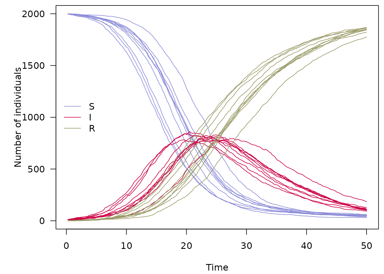
Adding age structure to the model
Adding age structure to the model consists of the following steps, which turn variables into arrays:
- Define the number of age categories as a user parameter
N_age. - Add age structure to each compartment, by adding square brackets to the lvalues.
- Modify the rvalues to use quantities from the appropriate
compartment, by adding an
iindex to the rvalues. These will automatically be looped over. - Where an age compartment needs to be reduced into a single
compartment/variable, use
sum(or another array function from https://mrc-ide.github.io/odin/articles/functions.html as appropriate) - Define the dimensions of all arrays, for example by setting
dim(S) <- N_age.
This would simply give N_age independent processes
equivalent to the first model, scaled by the size of the population in
each age category. To actually make this useful, you likely want to add
some interaction or transitions between the compartments. An example of
this would be to add an age-specific contact matrix, demonstrated below,
which defines a different force of infection
for each age group. This is calculated by
In the odin code:
m[, ] <- user() # age-structured contact matrix
s_ij[, ] <- m[i, j] * I[i]
lambda[] <- beta / N * sum(s_ij[i, ])
The probability of infection of a susceptible is then indexed by this force of infection:
p_SI[] <- 1 - exp(-lambda[i] * dt)Putting this all together, the age structured SIR model is as follows:
## Definition of the time-step and output as "time"
dt <- user()
initial(time) <- 0
update(time) <- (step + 1) * dt

## Core equations for transitions between compartments:
update(S_tot) <- S_tot - sum(n_SI)
update(I_tot) <- I_tot + sum(n_SI) - sum(n_IR)
update(R_tot) <- R_tot + sum(n_IR)

## Equations for transitions between compartments by age group
update(S[]) <- S[i] - n_SI[i]
update(I[]) <- I[i] + n_SI[i] - n_IR[i]
update(R[]) <- R[i] + n_IR[i]

## To compute cumulative incidence
update(cumu_inc[]) <- cumu_inc[i] + n_SI[i]

## Individual probabilities of transition:
p_SI[] <- 1 - exp(-lambda[i] * dt) # S to I
p_IR <- 1 - exp(-gamma * dt) # I to R

## Force of infection
m[, ] <- user() # age-structured contact matrix
s_ij[, ] <- m[i, j] * I[i]
lambda[] <- beta * sum(s_ij[, i])

## Draws from binomial distributions for numbers changing between
## compartments:
n_SI[] <- rbinom(S[i], sum(p_SI[i]))
n_IR[] <- rbinom(I[i], p_IR)

## Initial states:
initial(S_tot) <- sum(S_ini)
initial(I_tot) <- sum(I_ini)
initial(R_tot) <- 0

initial(S[]) <- S_ini[i]
initial(I[]) <- I_ini[i]
initial(R[]) <- 0
initial(cumu_inc[]) <- 0

## User defined parameters - default in parentheses:
S_ini[] <- user()
I_ini[] <- user()
beta <- user(0.0165)
gamma <- user(0.1)

# dimensions of arrays
N_age <- user()
dim(S_ini) <- N_age
dim(I_ini) <- N_age
dim(S) <- N_age
dim(I) <- N_age
dim(R) <- N_age
dim(cumu_inc) <- N_age
dim(n_SI) <- N_age
dim(n_IR) <- N_age
dim(p_SI) <- N_age
dim(m) <- c(N_age, N_age)
dim(s_ij) <- c(N_age, N_age)
dim(lambda) <- N_age
As before, save the file, and use odin.dust to compile
the model:
gen_age <- odin.dust::odin_dust("sirage.R")
#> ℹ 21 functions decorated with [[cpp11::register]]
#> ✔ generated file cpp11.R
#> ✔ generated file cpp11.cpp
#> ℹ Re-compiling sirageae032191
#> ── R CMD INSTALL ───────────────────────────────────────────────────────────────
#> * installing *source* package ‘sirageae032191’ ...
#> ** using staged installation
#> ** libs
#> using C++ compiler: ‘g++ (Ubuntu 11.4.0-1ubuntu1~22.04) 11.4.0’
#> g++ -std=gnu++17 -I"/opt/R/4.4.1/lib/R/include" -DNDEBUG  -I'/home/runner/work/_temp/Library/cpp11/include' -I/usr/local/include   -I"/home/runner/work/_temp/Library/dust/include" -DHAVE_INLINE -fopenmp  -fpic  -g -O2  -Wall -pedantic -fdiagnostics-color=always  -c cpp11.cpp -o cpp11.o
#> g++ -std=gnu++17 -I"/opt/R/4.4.1/lib/R/include" -DNDEBUG  -I'/home/runner/work/_temp/Library/cpp11/include' -I/usr/local/include   -I"/home/runner/work/_temp/Library/dust/include" -DHAVE_INLINE -fopenmp  -fpic  -g -O2  -Wall -pedantic -fdiagnostics-color=always  -c dust.cpp -o dust.o
#> g++ -std=gnu++17 -shared -L/opt/R/4.4.1/lib/R/lib -L/usr/local/lib -o sirageae032191.so cpp11.o dust.o -fopenmp -L/opt/R/4.4.1/lib/R/lib -lR
#> installing to /tmp/RtmpYG5M0v/devtools_install_193b3d68ce6a/00LOCK-file193b4e80506b/00new/sirageae032191/libs
#> ** checking absolute paths in shared objects and dynamic libraries
#> * DONE (sirageae032191)
#> ℹ Loading sirageae032191
We can generate an age-structured contact matrix based on the POLYMOD survey by using the socialmixr package:
data(polymod, package = "socialmixr")

## In this example we use 8 age bands of 10 years from 0-70 years old.
age.limits = seq(0, 70, 10)

## Get the contact matrix from socialmixr
contact <- socialmixr::contact_matrix(
  survey = polymod,
  countries = "United Kingdom",
  age.limits = age.limits,
  symmetric = TRUE)
#> Removing participants that have contacts without age information. To change this behaviour, set the 'missing.contact.age' option

## Transform the matrix to the (symetrical) transmission matrix
## rather than the contact matrix. This transmission matrix is
## weighted by the population in each age band.
transmission <- contact$matrix /
  rep(contact$demography$population, each = ncol(contact$matrix))
transmission
#>       contact.age.group
#>              [0,10)      [10,20)      [20,30)      [30,40)      [40,50)
#>   [1,] 7.347226e-07 1.680174e-07 1.621901e-07 2.521672e-07 1.256518e-07
#>   [2,] 1.680174e-07 1.035454e-06 1.691176e-07 1.696640e-07 2.180115e-07
#>   [3,] 1.621901e-07 1.691176e-07 4.700903e-07 2.054877e-07 2.068876e-07
#>   [4,] 2.521672e-07 1.696640e-07 2.054877e-07 3.115246e-07 2.230430e-07
#>   [5,] 1.256518e-07 2.180115e-07 2.068876e-07 2.230430e-07 3.351858e-07
#>   [6,] 8.032478e-08 1.038464e-07 1.798672e-07 1.677531e-07 1.756190e-07
#>   [7,] 8.147558e-08 6.984139e-08 1.164168e-07 1.497579e-07 1.456498e-07
#>   [8,] 2.987539e-08 7.531256e-08 5.961167e-08 4.627471e-08 1.247385e-07
#>       contact.age.group
#>             [50,60)      [60,70)          70+
#>   [1,] 8.032478e-08 8.147558e-08 2.987539e-08
#>   [2,] 1.038464e-07 6.984139e-08 7.531256e-08
#>   [3,] 1.798672e-07 1.164168e-07 5.961167e-08
#>   [4,] 1.677531e-07 1.497579e-07 4.627471e-08
#>   [5,] 1.756190e-07 1.456498e-07 1.247385e-07
#>   [6,] 2.472049e-07 1.650819e-07 1.074040e-07
#>   [7,] 1.650819e-07 2.008121e-07 1.427706e-07
#>   [8,] 1.074040e-07 1.427706e-07 1.931392e-07
This can be given as a parameter to the model by adding the argument
pars = list(m = transmission) when using the
new() method on the gen_age generator.
N_age <- length(age.limits)
n_particles <- 5L
dt <- 0.25
model <- gen_age$new(pars = list(dt = dt,
                                 S_ini = contact$demography$population,
                                 I_ini = c(0, 10, 0, 0, 0, 0, 0, 0),
                                 beta = 0.2 / 12.11,
                                 gamma = 0.1,
                                 m = transmission,
                                 N_age = N_age),
                     time = 1,
                     n_particles = n_particles,
                     n_threads = 1L,
                     seed = 1L)

# Define how long the model runs for, number of time steps
n_times <- 1000

# Create an array to contain outputs after looping the model.
# Array contains 35 rows = Total S, I, R (3), and
# in each age compartment (24) as well as the cumulative incidence (8)
x <- array(NA, dim = c(model$info()$len, n_particles, n_times))

# For loop to run the model iteratively
for (t in seq_len(n_times)) {
  x[ , , t] <- model$run(t)
}
time <- x[1, 1, ]
x <- x[-1, , ]
# Plotting the trajectories
par(mfrow = c(2,4), oma=c(2,3,0,0))
for (i in 1:N_age) {
  par(mar = c(3, 4, 2, 0.5))
  cols <- c(S = "#8c8cd9", I = "#cc0044", R = "#999966")
  matplot(time, t(x[i + 3,, ]), type = "l", # Offset to access numbers in age compartment
          xlab = "", ylab = "", yaxt="none", main = paste0("Age ", contact$demography$age.group[i]),
          col = cols[["S"]], lty = 1, ylim=range(x[-1:-3,,]))
  matlines(time, t(x[i + 3 + N_age, , ]), col = cols[["I"]], lty = 1)
  matlines(time, t(x[i + 3 + 2*N_age, , ]), col = cols[["R"]], lty = 1)
  legend("right", lwd = 1, col = cols, legend = names(cols), bty = "n")
  axis(2, las =2)
}
mtext("Number of individuals", side=2,line=1, outer=T)
mtext("Time", side = 1, line = 0, outer =T)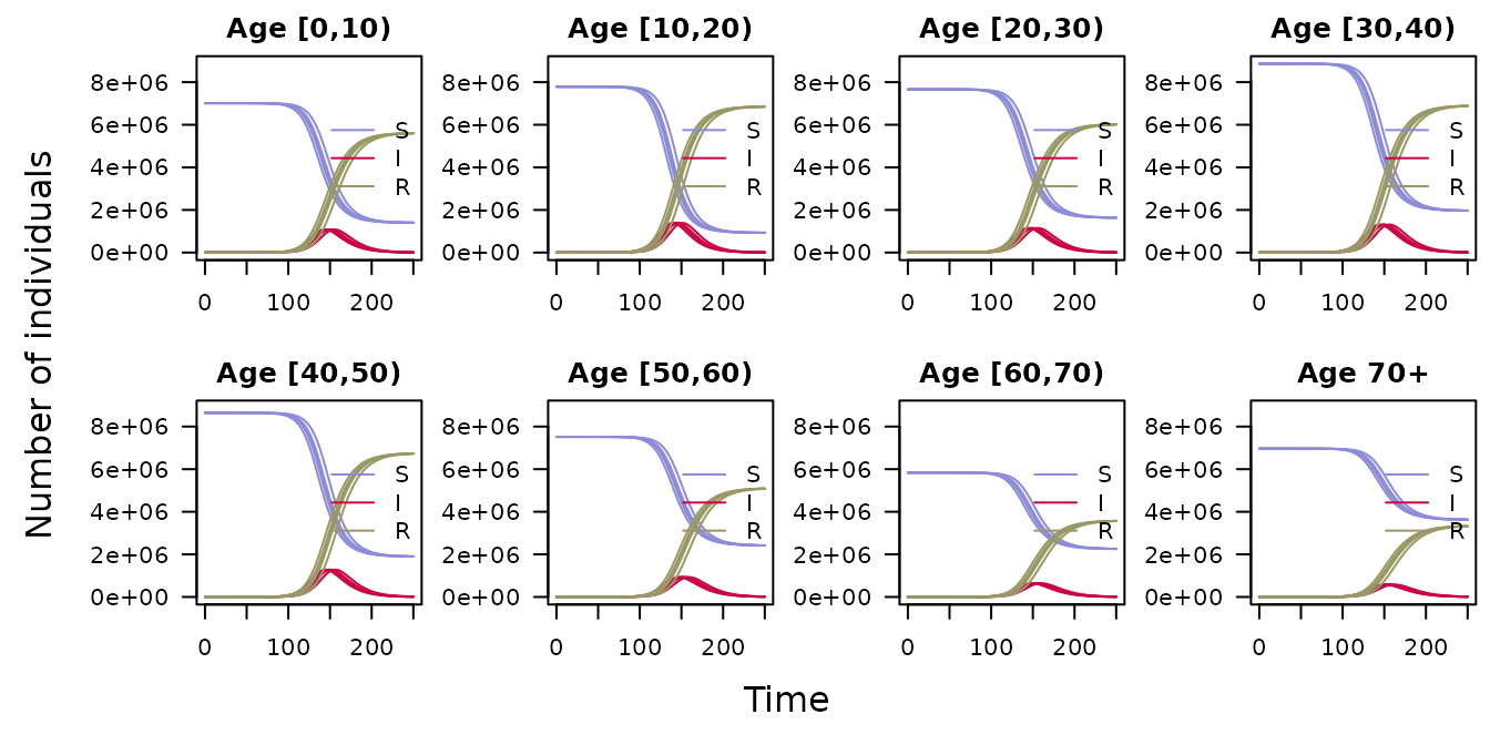
Note that a scale factor is introduced for beta so that
remains at 2, offsetting the scaling of the contact matrix
m. This is calculated using the next-generation matrix. See
Driessche and Towers and
Feng.
Many other methods are available on the dust object to support
inference, but typically you may want to use the mcstate
package instead of calling these directly. However, if you wish to
simulate state space models with set parameters, this can be done
entirely using the commands above from dust.