Porting from odin

odin.dust is built on odin, and so many models will work without modification, however there are some differences.

discrete-time models may not use output() (this is allowed for ODE models)
models may not use interpolate()
delays are not supported
not all stochastic distributions are supported
there are some interface tweaks that follow from using dust as the engine

There are some big advantages though in using odin.dust instead of the stochastic model support in odin:

models can run in parallel, which provides a near linear speed up in the number of cores
your model can be easily used in the particle filter and pmcmc machinery of mcstate
dust provides machinery for working with multiple realisations at once
odin.dust allows “mixed” models where most of the dynamics come from a set of ODEs but with periodic stochastic perturbations

Below, we describe how to address the most common issues when updating dust models to use odin.dust

Avoiding `output()`

(This section applies only to discrete time models, you can use output() freely in ODE models as in odin)

In odin you can write:

gen <- odin::odin({
  initial(x) <- 1
  update(x) <- x + 1
  output(y) <- x / 2
})

and use this to create a model where you have one input variable (on which the system depends) and one output variable (entirely derived from the inputs).

gen$new()$run(0:5)
#>      step x   y
#> [1,]    0 1 0.5
#> [2,]    1 2 1.0
#> [3,]    2 3 1.5
#> [4,]    3 4 2.0
#> [5,]    4 5 2.5
#> [6,]    5 6 3.0

This is important in ODE models because there are often things that you want to observe that are functions of the system but for which you can’t write out equations to describe them in terms of their rates - the sum over a set of variables for example.

Note here how the x used in the calculation is really the x at the end of a time step, not the x on inputs, which means that the output column satisfies y == x / 2. This turns out to be very hard to get right and reason about, and involves some fairly unpleasant bookkeeping in dde; in effect we run an additional time step at the end of the run in order to compute these output variables, and that is inefficient for dust’s use within a particle filter.

More importantly, there is no great need for output for discrete time models, as we can treat y above as just another variable. This also allows us to be more explicit about when within the time step this output is being computed:

gen <- odin.dust::odin_dust({
  initial(x) <- 1
  new_x <- x + 1
  update(x) <- new_x
  initial(y1) <- 0
  initial(y2) <- 0
  update(y1) <- x / 2
  update(y2) <- new_x / 2
})

We will probably deprecate these in odin for discrete time model because these turned out to be hard to get right - we need to compute the output variables at the end of the time step, which lead to confusion about which x was being read - the x at the beginning of the time step or the x at the end. This is implemented by some fairly unpleasant bookkeeping that we would like to drop.

t(drop(gen$new(list(), 0, 1)$simulate(0:5)))
#>      [,1] [,2] [,3]
#> [1,]    1  0.0  0.0
#> [2,]    2  0.5  1.0
#> [3,]    3  1.0  1.5
#> [4,]    4  1.5  2.0
#> [5,]    5  2.0  2.5
#> [6,]    6  2.5  3.0

Here, the first column is x as in the first column. The second column computes the relationship with the x at the beginning of the time step, while the third is most equivalent to our previous output command and requires storing the that will become the updated x in order to use that value to both update x and y2.

Limited support for `interpolate()`

This is supported for ODE models, though only for interpolating scalar outputs (this was by far the most common use case).

Interpolation is not supported for discrete time models. For these models, we recommend doing the interpolation as part of your parameter preparation and passing in an expanded vector which you then look up. This also makes it (somewhat) more obvious how time is being treated in your model.

For an example, here’s a model of logistic growth in discrete time, where the carrying capacity varies seasonally, implemented as a piecewise-constant interpolation between some points. It’s easy enough to create some sort of time varying time series to use:

t_capacity <- seq(0, 100, by = 10)
y_capacity <- runif(length(t_capacity), 100, 200)

Somewhat awkwardly, the step number here will be used as the “time” variable (vs within an ODE model where there’s much more of a concept of time).

gen <- odin::odin({
  initial(n) <- 1
  update(n) <- (1 + r * (1 - n / K)) * n
  r <- user(0.5)
  K <- interpolate(t_capacity, y_capacity, "constant")
  t_capacity[] <- user()
  y_capacity[] <- user()
  dim(t_capacity) <- user()
  dim(y_capacity) <- user()
})

Then run this model

pars <- list(t_capacity = t_capacity, y_capacity = y_capacity)
mod <- gen$new(user = pars)
plot(mod$run(0:100), type = "s")
lines(t_capacity, y_capacity, type = "s", col = "red", lty = 2)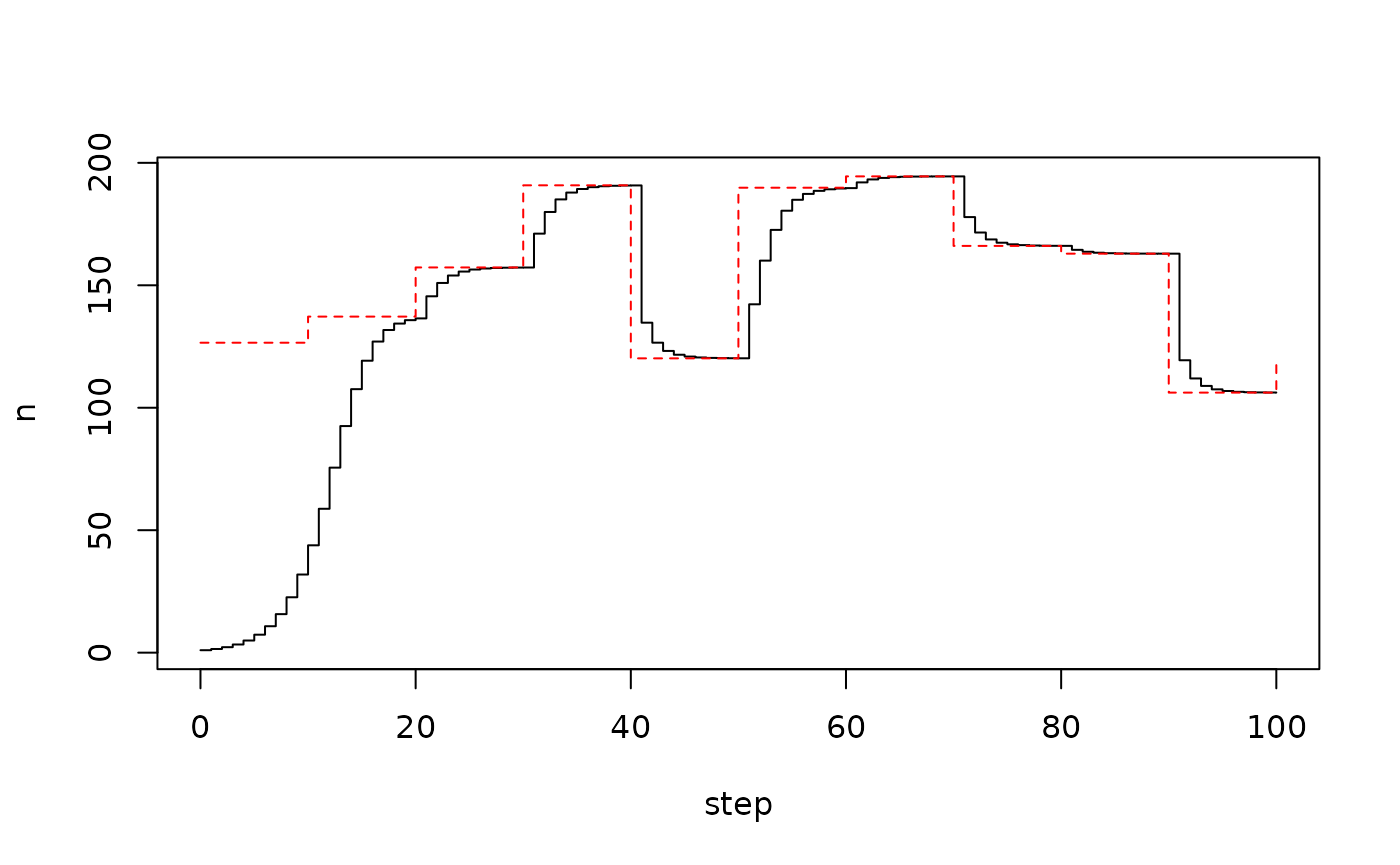

Everything is unambiguous for a continuous time model, but here it’s not so clear - when we do the lookup with step, what are we finding?

The other complication arises when you want to rescale time, so that each step has a size of dt and then you want to think about interpolation in this new time variable; for example

gen <- odin::odin({
  initial(n) <- 1
  update(n) <- (1 + r * dt * (1 - n / K)) * n
  initial(time) <- 0
  update(time) <- time + dt # or equivalently (step + 1) * dt
  r <- user(0.5)
  dt <- user(0.25)
  K <- interpolate(t_capacity, y_capacity, "constant")
  t_capacity[] <- user()
  y_capacity[] <- user()
  dim(t_capacity) <- user()
  dim(y_capacity) <- user()
})

Here, we scale the rate of change r by our dt parameter, and we output a new variable time which keeps track of our rescaling. Once we do this we need to also rescale the times used in the interpolation.

Our current workaround is to create a full set of interpolated values by step as a parameter, using one of R’s interpolation functions. To look up the value, we use

K_step[] <- user()
dim(K_step) <- user()
K <- if (as.integer(step) >= length(K)) K[length(K)] else K[step + 1]

which looks up the value of K from a fully expanded set, falling back on returning the last value for any steps beyond the end of the series. Here, step can be translated into time by step * dt and at the end of the step time will have this value (so this value of K is used in the move from step - 1 to step).

Delays are not supported

Delays have never really been supported for discrete time models in odin, but they are useful for ODE models. Our DDE solver is extremely basic and is unlikely to do well with ODEs that use stochasticity (see below), so we have chosen not to expose it in dust.

One potential use of delays in discrete time models is to allow computing incidence from prevalence. Suppose that you have some cumulative variable (say, number of total infections) and you want to compute the number of infections over some time period, you could compute this by doing

total <- total + new           # accumulating variable
total_lag <- delay(total, 10)  # lag of the variable total by 10 time steps
incidence <- total - total_lag # number of events in the last 10 time steps

This is particularly useful for models where you are fitting to incidence data.

Our suggested workaround to this is to use an accumulator variable that you reset based on a modulo of step with your interval

total <- total + new
initial(incidence) <- 0
update(incidence) <- if (step %% 10 == 0) new else incidence + new

Not all distributions are supported

For stochastic models, odin.dust uses dust for random numbers, which has the big advantage that they can be computed in parallel. The disadvantage is that it does not support the full set of distributions implemented in R and therefore available to odin

Supported distributions:

binomial (rbinom)
exponential (rexp)
normal (rnorm)
gamma (rgamma)
hypergeometric (rhyper)
negative binomial (rnbinom)
Poisson (rpois)
uniform (unif)

Unsupported distributions:

beta (rbeta)
non-central beta (rnbeta)
Cauchy (rcauchy)
chi-squared (chisq)
non-central chi-squared (rnchisq)
F (rf)
non-central F (rnf)
geometric (rgeom)
logistic (rlogis)
lognormal (rlnorm)
Student’s t (rt)
non-central t (rnt)
Weibull (rweibull)
Wilcoxon rank sum (rwilcox)
Wilcoxon signed rank (rsignrank)

There are two special cases, for the multinomial (rmultinom) and the multivariate hypergeometric (rmhyper; not available in R but available in odin). These are both available in a limited form in odin, where you can use them where the left hand side is a vector

prob[] <- user()
y[] <- rmultinom(size, prob)

where size is the number of trials and prob is a normalised vector of probabilities of success in each of the length(prob) classes. Note that y, the outcome, must have the same length of prob.

This is quite limiting as you cannot assign a sample as a row into a matrix or higher-dimensional structure. We have plans to improve this in odin itself (see #134, #213 and #255) but do not anticipate that this will be implemented in the short term.

In the binomial case you can rewrite the multinomial sampling as a series of binomials, for example the above expression could be rewritten

y[1] <- rbinom(size, prob[1])
y[2:length(y)] <- rbinom(size - sum(y[1:(i - 1)]), prob[i] / sum(prob[i:length(y)]))

A similar transform is possible for the multivariate hypergeometric from the hypergeometric (see odin’s rmhyper implementation for details).

Interface differences

These differences all follow from design decisions in dust.

The model is much more stateful. In odin, you create a model object and use that to run a simulation over some time steps. With dust you create a model and can advance it to a point in the simulation, then retrieve state, reorder particles (individual realisations), or update state, then continue. See this vignette for more information.

The model size cannot be changed after initialisation. While you can update parameters (via the $update_state method), it is an error if this changes the size of the state vector. This allows us to be much more efficient in terms of allocations, and is important to support the stateful interactions.

There is an assumption that more than one realisation is generally wanted. With discrete time and stochastic models in odin, the interface matches that of the ODE solver where we assume you’re interested in a single solution to a set of equations. With odin.dust (via dust) we assume that you are interested in a set of realisations, and so the return types have been structured with a “particle” dimension to make this easier. This also has the effect of moving time into the last dimensions of any returned data, not the first as in odin.

Compilation is much slower. This does make iteration over models more tedious, unfortunately. The slower compilation is a function of using C++ with a reasonable amount of template metaprogramming.

Avoiding output()

Limited support for interpolate()

Delays are not supported

Not all distributions are supported

Interface differences

Avoiding `output()`

Limited support for `interpolate()`