Basic tutorial
Keith Fraser and Bob Verity
2020-01-13
basic-tutorial.RmdThis vignette goes through a basic RMAPI analysis, using simulated data to test different methods. It covers:
- Simulating/loading data into R
- Creating a project and binding data to the project
- Creating a hex-map and checking coverage
- Running simulations
- Plotting results
- Repeat analysis using an explicit fitted model
Simulating/loading data
RMAPI uses pairwise information (i.e. statistics) between a series of spatial nodes (i.e. observations) to test for areas of significant spatial discontinuity. Therefore, the basic inputs to RMAPI are: 1) coordinates of nodes, 2) values of pairwise statistics. Node coordinates need to be in dataframe format, with two columns: long and lat, and pairwise statistics need to be formatted as a square matrix.
For the sake of this vignette we will use built-in functions to simulate data in the correct format with known spatial barriers. First, we will generate node coordinates uniformly at random over the sampling region. This is intended to represent a situation where we do not have control over sampling locations and therefore cannot create a perfect sampling grid - for example when sampling from major cities:
# Define coordinates of nodes
node_df <- data.frame(long = runif(100, -1.548, -1.478), lat = runif(100, 53.347, 53.379))
Next we create a list of polygons that represent barriers to gene flow. Each element of this list should be a dataframe specifying the coordinates of a polygon, which must make a complete ring (i.e. the final pair of longitude/latitude values must be identical to the first). We also need to define the penalty associated with each barrier, which acts as a multiplier to the intersection distance when calculating pairwise data (see below):
# Define barriers
barrier_list <- list()
barrier_list[[1]] <- data.frame(long = c(-1.54, -1.51, -1.49, -1.5, -1.535, -1.54),
                                lat = c(53.365, 53.37, 53.365, 53.36, 53.36, 53.365))
barrier_penalty <- 5
We can now simulate statistical values between nodes. The barrier_method = 2 method used here draws a straight line between nodes and calculates the intersection with barrier polygons before applying the barrier penalty per unit intersection, meaning that lines which go long-ways through a barrier experience a greater penalty. We also use dist_transform = 2 here, which assumes that values fall off exponentially with distance with rate lambda. Finally, random error is applied to all pairwise statistics in the form of Gaussian noise with standard deviation eps. Further details of barrier penalty methods and transformations can be found in the help for the sim_simple() function.
# Simulate pairwise statistics
sim_stat <- sim_simple(node_long = node_df$long,
                       node_lat = node_df$lat,
                       barrier_list = barrier_list,
                       barrier_penalty = barrier_penalty,
                       barrier_method = 2,
                       dist_transform = 2,
                       lambda = 50,
                       eps = 0.2)
When loading data from a file, it should be in the same format as this simulated data.
Creating a project and binding data
RMAPI works using projects, which are essentially just lists containing all data, input and outputs in one place. We can create a new project, and then bind our data to the project:
# Create new RMAPI project
p <- rmapi_project()
# bind data
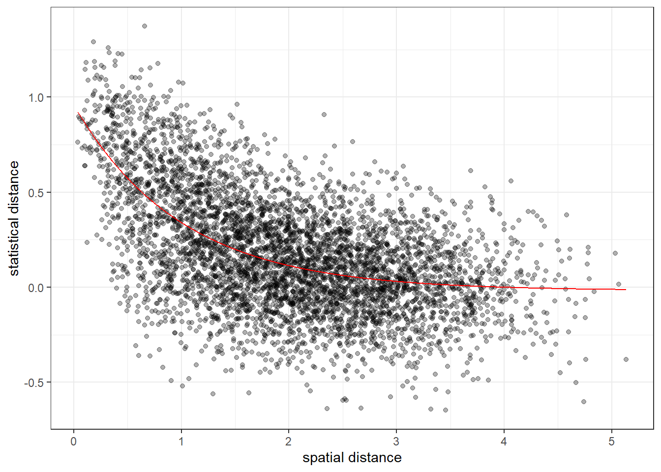
p <- bind_data(p, node_df$long, node_df$lat, sim_stat)Once we have data bound to a project we can use the plot_dist() function to explore the basic relationship between distance and pairwise statistical values:
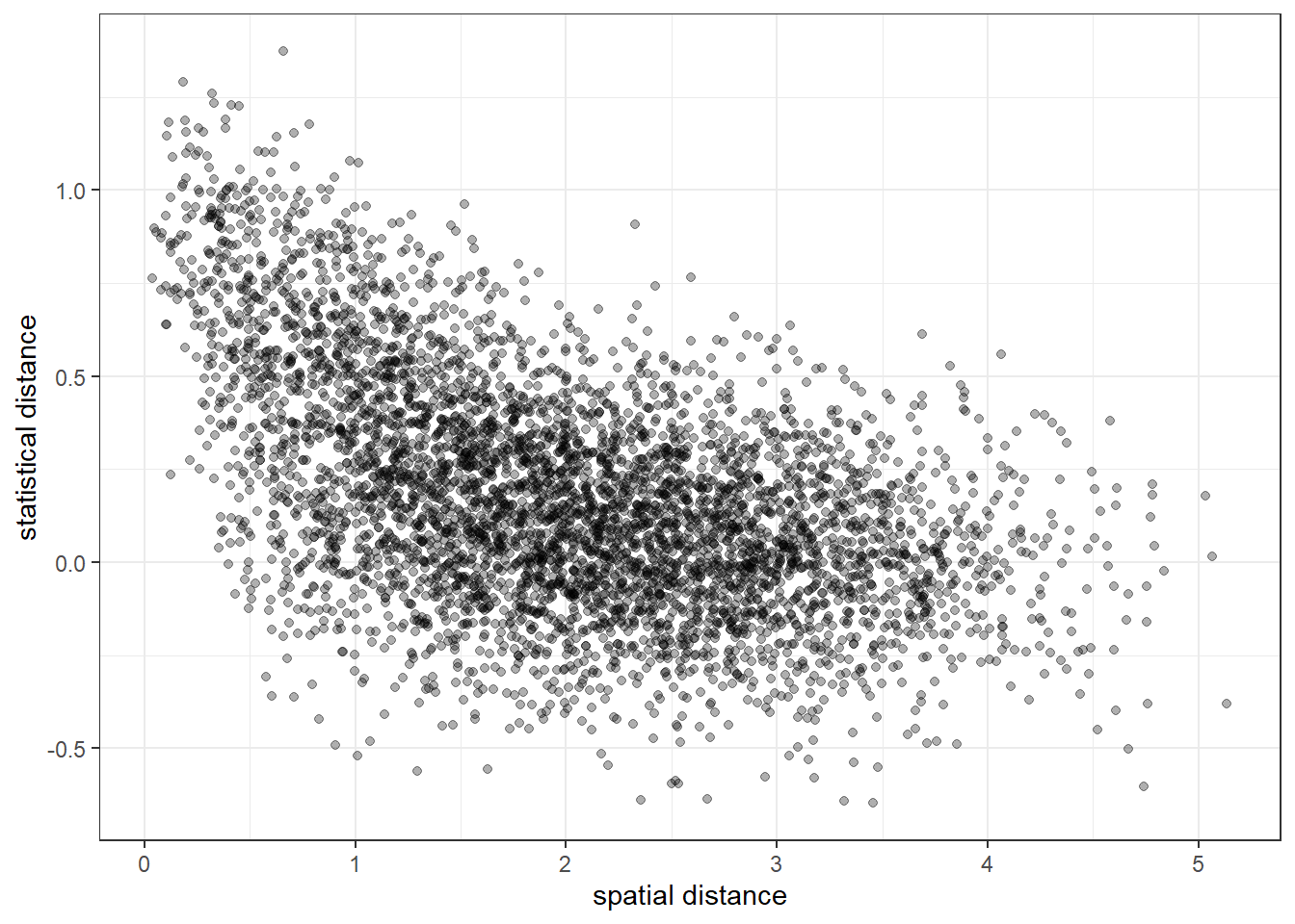
We can see the general shape of exponential fall-off, which we should expect from our simulation parameters, but the noise makes it very difficult to see if there are any more subtle patterns, e.g. spatial barriers.
Creating a hex map and testing coverage
Next, we need to create a hex-map:
## Creating hex map## 588 hexagons createdOnce we have a hex map we can use it to explore different values of the ellipse eccentricity used in the RMAPI method. An eccentricity of 1 defines a straight line between points, and an eccentricity of 0 represents a perfect circle. Whatever our chosen value, we should ensure that the number of ellipses intersecting each hex (the “coverage”) is sufficient to reduce noise, and increase reliability of the permutation testing procedure. We suggest that a minimum coverage of 100 is a good rule of thumb:
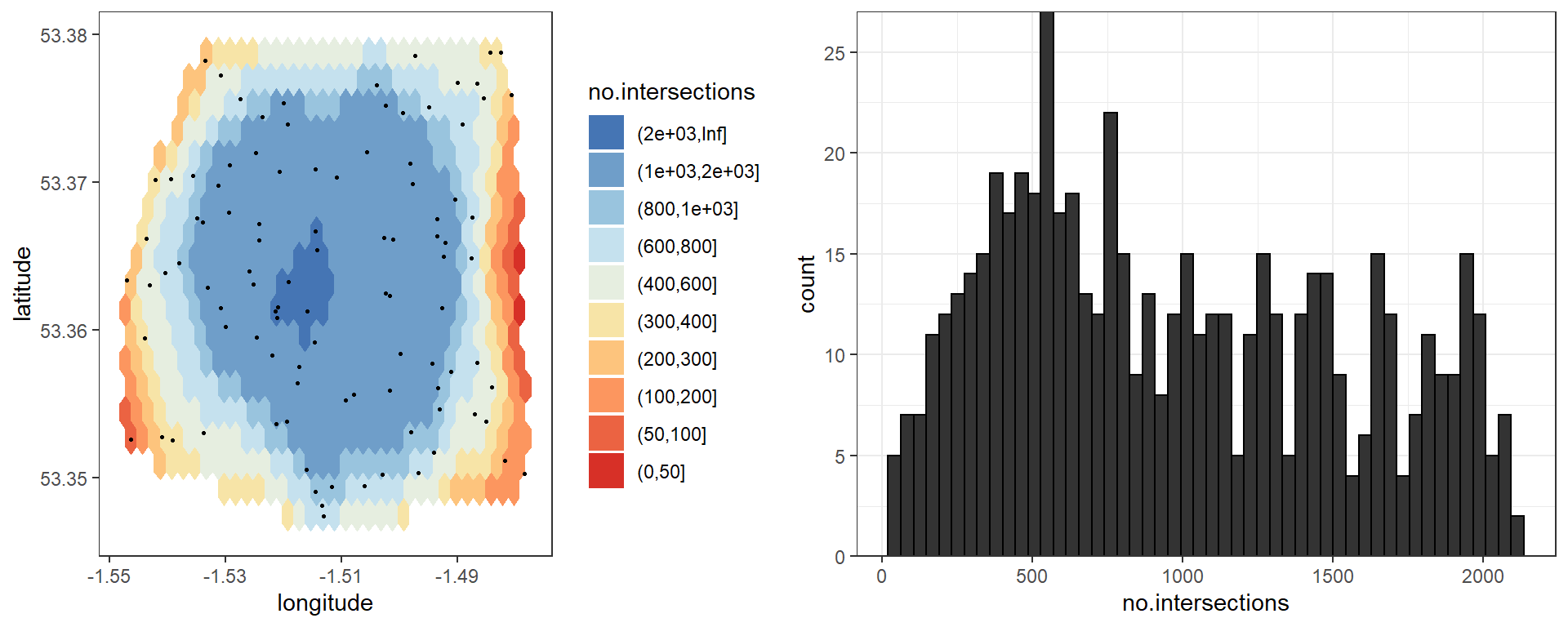
Here we can see that an eccentricity of 0.9 provides good coverage over most of the map, although we should be wary of values on the far East-West edges.
Running simulations
Now we are ready to run simulations. The following command computes hex values from pairwise statistics, and compares this map against a series of analogous maps produced after first permuting edge values. The output of this function includes the raw hex values, along with the rank of the raw hex values through the list of permutations (as a proportion). Note that for the sake of this vignette we use the report_progress = FALSE argument to avoid printing too much output, but you should run without this argument.
# Generate hex values
p <- rmapi_analysis(p, n_perms = 1e3, eccentricity = 0.9, n_breaks = 1, report_progress = FALSE)
## Loading data and parameters
## Setting up ellipses
## Computing map
## Running permutation testWe can use the plot_map() function to produce simple plots of the raw hex values, and the hex ranks:
# Plot hex values
plot1 <- plot_map(p, barrier_list = barrier_list)

# Plot hex ranks
plot2 <- plot_map(p, variable = "hex_ranks", barrier_list = barrier_list)

# Use gridExtra package to arrange ggplot objects
library(gridExtra)
grid.arrange(plot1, plot2, ncol = 2)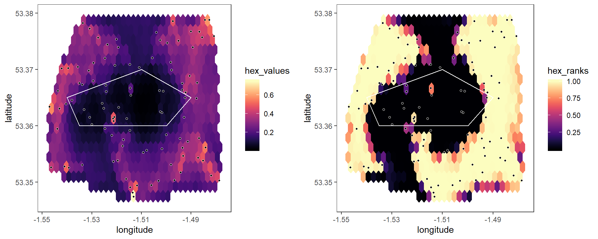
Notice from the hex map that values tend to be higher when nodes are close together - this occurs because of our assumed fall-off of statistical values with distance in our simulations. However, our null model for the permutation test is that there is no association between pairwise statistics and edges, and hence no spatial trend whatsoever, which is clearly not the case here. When we look at the hex ranks from the permutation test, this gives the appearance of artificial areas of significant spatial discontinuity, when in fact these are simply poorly-sampled areas. This is exactly the problem that RMAPI was designed to solve through the use of more refined permutation testing and null models. Several approaches are available to deal with this issue.
Distance-sensitive permutation
First, we can re-run the simulations, this time using a value of n_breaks = 20. This divides all edges into bins based on their spatial separation, and permutation testing then only occurs within bins - for example, pairwise values between nodes with short distances between them are only compared against values between other nodes with small separation distances, not against values between nodes with large separation distances:
# Generate hex values
p <- rmapi_analysis(p, n_perms = 1e3, eccentricity = 0.9, n_breaks = 20, report_progress = FALSE)
## Loading data and parameters
## Setting up ellipses
## Computing map
## Running permutation test# Plot hex values
plot1 <- plot_map(p, barrier_list = barrier_list)
# Plot hex ranks
plot2 <- plot_map(p, variable = "hex_ranks", barrier_list = barrier_list)
# Use gridExtra package to arrange ggplot objects
grid.arrange(plot1, plot2, ncol = 2)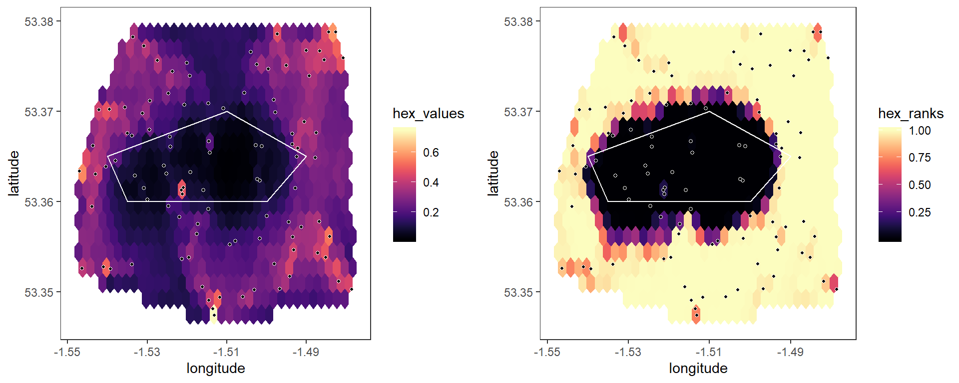
Now, although the raw map is the same, the hex ranks give a far more accurate pattern because they account for the natural trend with distance.
We can also produce an interactive map, making it easier to see how discontinuities may correspond to geographic features:
Fitting a distance dependence model
The second method implemented in RMAPI is to fit a specific model to the relationship between pairwise values and spatial distance and using model-generated values as a null data set. We can use the fit_model() function to fit either a linear model (type = 1) or an exponential model (type = 2). Clearly based on the pattern in the data we would want the exponential model in this example:
When running simulations with null_method = 2, the model fit is subtracted from the pairwise values, and the permutation testing procedure is then carried out on the residuals. This is slightly less flexible than the previous method, in that we must have an idea of the specific relationship between distance and statistical value, but can be more powerful as a result:
# Generate hex values
p <- rmapi_analysis(p, null_method = 2, n_perms = 1e3, eccentricity = 0.9, n_breaks = 1, report_progress = FALSE)
## Loading data and parameters
## Setting up ellipses
## Computing map
## Running permutation test# Plot hex values
plot1 <- plot_map(p, barrier_list = barrier_list)
# Plot hex ranks
plot2 <- plot_map(p, variable = "hex_ranks", barrier_list = barrier_list)
# Use gridExtra package to arrange ggplot objects
grid.arrange(plot1, plot2, ncol = 2)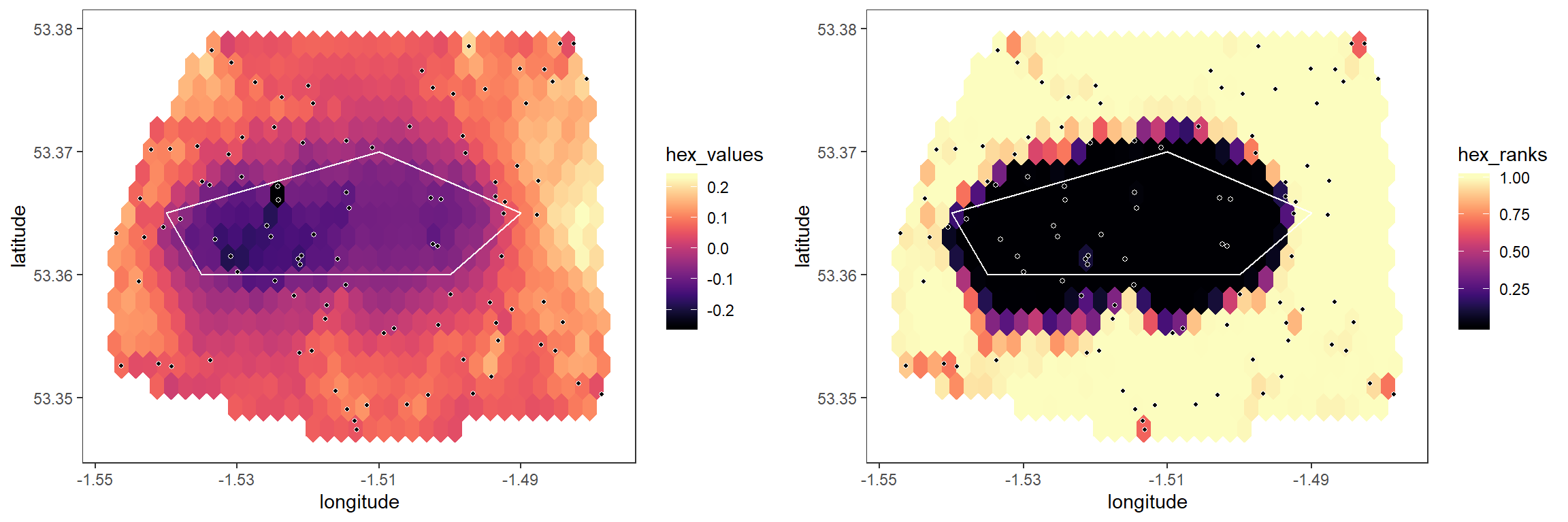
Note that there is nothing to stop us running the above procedure with n_breaks > 1, in which case the spatial permutation test is carried out on residuals, which could be useful if we believe our model is only a rough description of the actual relationship.