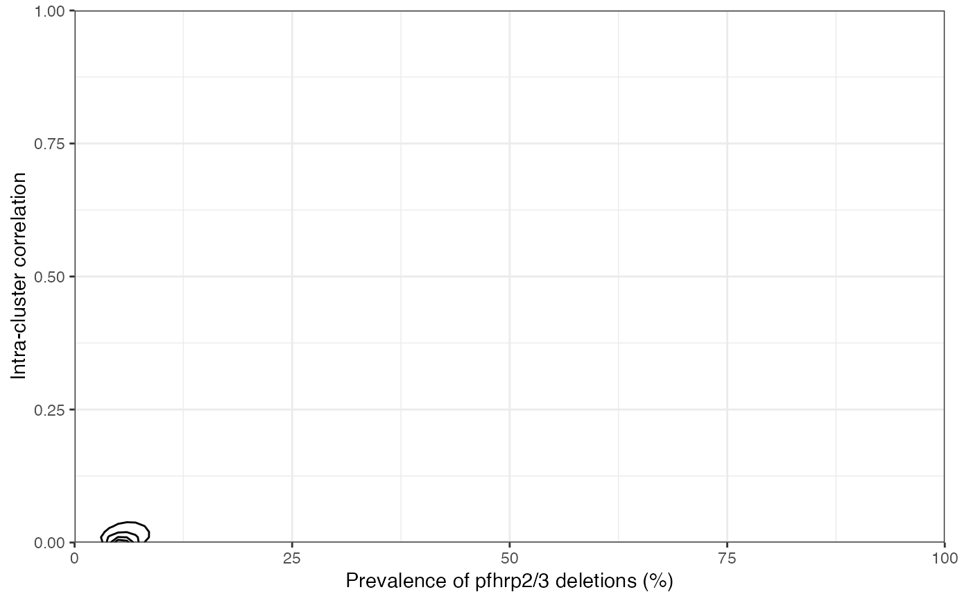
Runs get_joint() to obtain the joint posterior
distribution of the prevalence and the ICC. Creates a ggplot contour plot
object from this result.
Arguments
- n, N
the numerator (
n) and denominator (N) per cluster. These are both integer vectors.- prior_prev_shape1, prior_prev_shape2, prior_ICC_shape1, prior_ICC_shape2
parameters that dictate the shape of the Beta priors on prevalence and the ICC. See the Wikipedia page on the Beta distribution for more detail. The default values of these parameters were chosen based on an analysis of historical pfhrp2/3 studies, although this does not guarantee that they will be suitable in all settings.
- prev_breaks, ICC_breaks
the values at which to evaluate the posterior in both dimensions. Prevalence is returned in columns, ICC in rows.
- n_bins
the number of equally spaced breaks in the contour plot. For example, 5 bins creates 4 contour lines at 20%, 40%, 60% and 80% of the maximum value.