New Fitting Method: Rt Optimisation
rt_optimise.RmdThis vignette describes the new fitting method where we optimise the \(R_t\) values for a set of given parameters.
Method Outline
Descriptive
Inputs are assumed to be a set of distributions for the non \(R_t\) parameters and a set of deaths that occur over set time periods, so \(D_i\) deaths occur over the time period \([t_{f,i}, t_{s,i}]\) for each \(i \in 1\) to \(T_D\). We assume that the epidemic begins at time 0. We define our parameters to vary in the fitting process as \(\boldsymbol{R} = \{R_t;\ t\in 0\mathrm{\ to\ }T_R\}\). Each \(R_t\) to comes into effect at time \(t_{R_t}\), by default this every 14 days with \(T_R = T_D - \max{\boldsymbol{\lambda}}\).
- Generate \(N\) samples from our assumed distributions on our non \(R_t\) parameters. This will be discussed more in the section on Parameter Uncertainty.
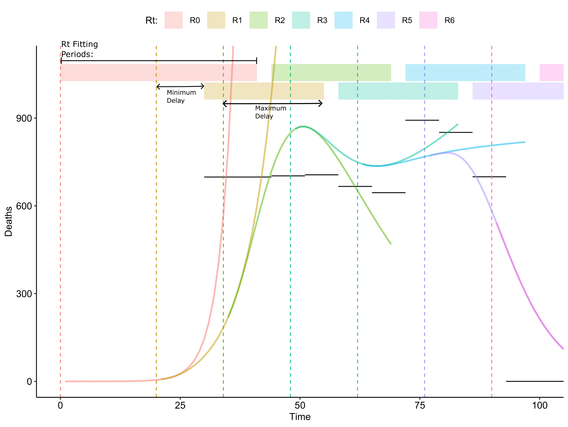
- Determine which deaths will be used to fit each \(R_t\). Using the structure of the model we calculate the average time from infection to death (given death is the outcome). This should match the delay between the \(R_t\) value changing and its effect on the modelled deaths. This value depends on the duration parameters given to the model and on the number of hospital or ICU beds available, hence we determine all 4 possible durations, \(\boldsymbol{\lambda}\). We define the relevant deaths for an \(R_t\) by choosing all deaths that lie within widest possible window that our \(R_t\) value could directly effect, meaning any death that has its entire time period occur within the bounds \([t_{R_t} + \min(\boldsymbol{\lambda}), t_{R_{t+1}} + \max(\boldsymbol{\lambda})]\).
- For \(R_0\) we set the bounds to \([0, t_{R_{1}} + \max(\boldsymbol{\lambda})]\), and for \(R_{T_R}\) we set the bounds to \({t_{R_{T_R}} + \min(\boldsymbol{\lambda}), t_{s,T_D}}\).
- For simplity we will define \(\boldsymbol{i_{R_t}} = \{i;\ t_{s,i} \geq t_{R_t} + \min(\boldsymbol{\lambda})\ \&\ t_{f,i} \leq \max(\boldsymbol{\lambda})\}\), which is the indexes of all deaths that occur within \(R_t\)’s fitting period
- For each distinct sample from the parameter distributions:
- Begin the estimation procedure by estimating \(R_0\) and \(I_0\), the initial number of infections. \(I_0\) is uniformly spread across the unvaccinated working age population.
- When optimising \(R_t\) we set upper and lower bounds on the values it can take, which will be the hyper parameters \(\alpha, \beta\) with \(\alpha > \beta\) and \(\alpha = 10, \beta = 0.5\) by default. To optimise \(I_0\) we split a given range of numbers into \(N_p\) values, which we’ll call \(P_{I_0}\).
- To find our optimal values for \(R_0\) and \(I_0\) we optimise the log-likelihoods for each element of \(P_{I_0}\) in terms of \(R_t\) using the Brent optmisation method. The likelihood uses the negative binomial distribution with a mean equal to the modelled deaths and \(k\) a user defined dispersion parameter on \(D_i\), the deaths that fall within \(R_0\) fitting window as per step 2. We then take the \(I_0\) and \(R_t\) which the highest optimised likelihood as our values for \(R_0\) and \(I_0\).
- Using \(R_0\) and \(I_0\) we calculate the state of the models compartments at time \(t_{R_1}\), which we will call \(\boldsymbol{I_{R_1}}\).
- For each \(R_t \in \boldsymbol{R}/R_0\):
- Choose \(R_t\) by optimising the log-likelihood over all \(D_i\) such that \(i \in i_{R_t}\)
- With \(R_t\) and \(\boldsymbol{I_{R_t}}\) calculate \(\boldsymbol{I_{R_{t+1}}}\) which occurs at time \(t_{R_t + 1}\).
- Should end up with a set \(\boldsymbol{R}\) for each sample such that modelled deaths are similar to the observed deaths.
Mathematical
Let \(\boldsymbol{p}\) be a set of non-\(R_t\) model parameters. Then let \(m_{I}(\boldsymbol{p}, \boldsymbol{I_{R_{t}}}, R_t, t)\) be a function that returns the model state at time \(t\), given the state of the model when \(R_{t+1}\) comes into effect, and \(m_{d}(\boldsymbol{p}, \boldsymbol{I_{R_t}}, R_t, t_s, t_f)\) be a function that produces the number of deaths in the model occuring over time period \([t_s, t_f]\).
For each \(\boldsymbol{p}\):
- \[ \{R_0, I_0\} = \mathrm{argmax}_{x,y \in [\alpha, \beta] \times \boldsymbol{P_{I_0}}}\left( \prod_{i \in \boldsymbol{i_{R_0}}}\frac{\Gamma(D_i + n_i)}{\Gamma(n_i)D_i!}(1-p_i)^{D_i}p_i^{n_i} \right), \] where: \[ p_i = \frac{k}{k + \mu_i},\ n_i = \frac{p_i \times \mu_i}{1-p_i} ,\ \ \mu_i = m_d(\boldsymbol{p}, y, x, t_{s,i}, t_{f,i}). \]
- \(\boldsymbol{I_{R_1}} = m_I(\boldsymbol{p}, I_0, R_0, t_{R_1})\), note that we treat \(I_0\) and \(\boldsymbol{I_{R_0}}\) interchangeably here.
- For each element of \(\{t; t>0\ \&\ R_t \in [\alpha, \beta]\}\)
- \[ R_t = \mathrm{argmax}_{x \in \boldsymbol{P_{R_t}}}\left( \prod_{i \in \boldsymbol{i_{R_t}}}\frac{\Gamma(D_i + n_i)}{\Gamma(n_i)D_i!}(1-p_i)^{D_i}p_i^{n_i} \right) \] where: \[ p_i = \frac{k}{k + \mu_i},\ \ n_i = \frac{p_i \times \mu_i}{1-p_i},\ \ \mu_i = m_d(\boldsymbol{p}, \boldsymbol{I_{R_t}}, x, t_{s,i}, t_{f,i}). \]
- \(\boldsymbol{I_{R_{t+1}}} = m_I(\boldsymbol{p}, \boldsymbol{I_{R_{t}}}, R_t, t_{R_{t+1}})\)
Parameter Uncertainty
It is up to the user to setup the distributions on their parameters or just pass the function and set of parameters they like.
In the lmic_reports these are drawn from distributions representative of the epidemic, please see the methods page.
Limitations
It is necessary to bound \(R_t\) above and below certain thresholds to avoid dramatically high or low changes. So far all fits seem to work well with \(R_t\) ranges around \(0.5\) or \(0.9\) to \(10\), though it is possible for there be a curve that cannot be matched with this algorithm on simple bounds.