Squire Validation Run

Setup

Let’s compare safir to squire. Set up our parameters for running. We use a time step of 0.1 days. We use get_parameters to grab parameters directly from the squire package.

library(safir)
library(squire)
#> 
#> Attaching package: 'squire'
#> The following object is masked from 'package:safir':
#> 
#>     get_population
library(data.table)
library(ggplot2)
library(parallel)

iso3c <- "ATG"
contact_mat <- squire::get_mixing_matrix(iso3c = iso3c)
pop <- safir::get_population(iso3c)

# use as many as you want normally.
options("mc.cores" = 2)

nrep <- 10
# Scale it for speed
pop$n <- as.integer(pop$n / 5)

# Create our simulation parameters
R0 <- 2
time_period <- 200
dt <- 0.1

parameters <- get_parameters(
  population = pop$n,
  contact_matrix_set = contact_mat,
  iso3c = iso3c,
  R0 = R0,
  time_period = time_period,
  dt = dt
)

We’re going to compare it to squire. Let’s run that first.

out <- squire::run_explicit_SEEIR_model(
  population = pop$n,
  country = "Antigua and Barbuda",
  contact_matrix_set = contact_mat,
  time_period = time_period,
  replicates = nrep,
  day_return = TRUE,
  R0 = R0,
  dt = dt
)
#> Warning: 'explicit_SEIR(...)' is deprecated; please use 'explicit_SEIR$new(...)'
#> instead

Run safir

Now we can run safir in parallel. Note that the timesteps is the maximum day divided by the size of the step, dt.

To set up the model, first call create_variables which creates the categorical states and ages for the simulated population. Then create_events and attach_event_listeners creates the list of events and attaches listeners which handle state changes and queue future events. Next, a renderer objects is made. Note that because we are only outputting simulation state every day despite the time step size, the number of time steps is equal to the number of days, not the total number of time steps taken.

Next the list of processes can be made. We use infection_process_cpp which is a C++ version of infection_process to speed up the simulation. Tests are included in the package to ensure the same results are returned when using identical random number seeds. Finally the simulation can be run.

system.time(
  saf_reps <- mclapply(X = 1:nrep,FUN = function(x){
    
    timesteps <- parameters$time_period/dt
    variables <- create_variables(pop = pop, parameters = parameters)
    events <- create_events(parameters = parameters)
    attach_event_listeners(variables = variables,events = events,parameters = parameters, dt = dt)
    renderer <- individual::Render$new(parameters$time_period)
    processes <- list(
      infection_process_cpp(parameters = parameters,variables = variables,events = events,dt = dt),
      categorical_count_renderer_process_daily(renderer, variables$state, categories = variables$states$get_categories(),dt = dt)
    )
    setup_events(parameters = parameters,events = events,variables = variables,dt = dt)

    individual::simulation_loop(
      variables = variables,
      events = events,
      processes = processes,
      timesteps = timesteps
    )
    df <- renderer$to_dataframe()
    df$repetition <- x
    return(df)
  })
)
#>    user  system elapsed 
#>  20.077   0.144  20.811

Let’s organize our data for plotting. We’ll compare the 2.5th and 97.5th quantiles and median.

saf_reps <- do.call(rbind,saf_reps)

# safir
saf_dt <- as.data.table(saf_reps)
saf_dt[, IMild_count := IMild_count + IAsymp_count]
saf_dt[, IAsymp_count := NULL]
saf_dt <- melt(saf_dt,id.vars = c("timestep","repetition"),variable.name = "name")
saf_dt[, model := "safir"]
saf_dt[, name := gsub("(^)(\\w*)(_count)", "\\2", name)]
setnames(x = saf_dt,old = c("timestep","name","value"),new = c("t","compartment","y"))
saf_dt <- saf_dt[, .(ymin = quantile(y,0.025), ymax = quantile(y,0.975), y = median(y)), by = .(t,compartment,model)]

# squire
sq_dt <- as.data.table(squire::format_output(out, unique(saf_dt$compartment)))
sq_dt[, model := "squire"]
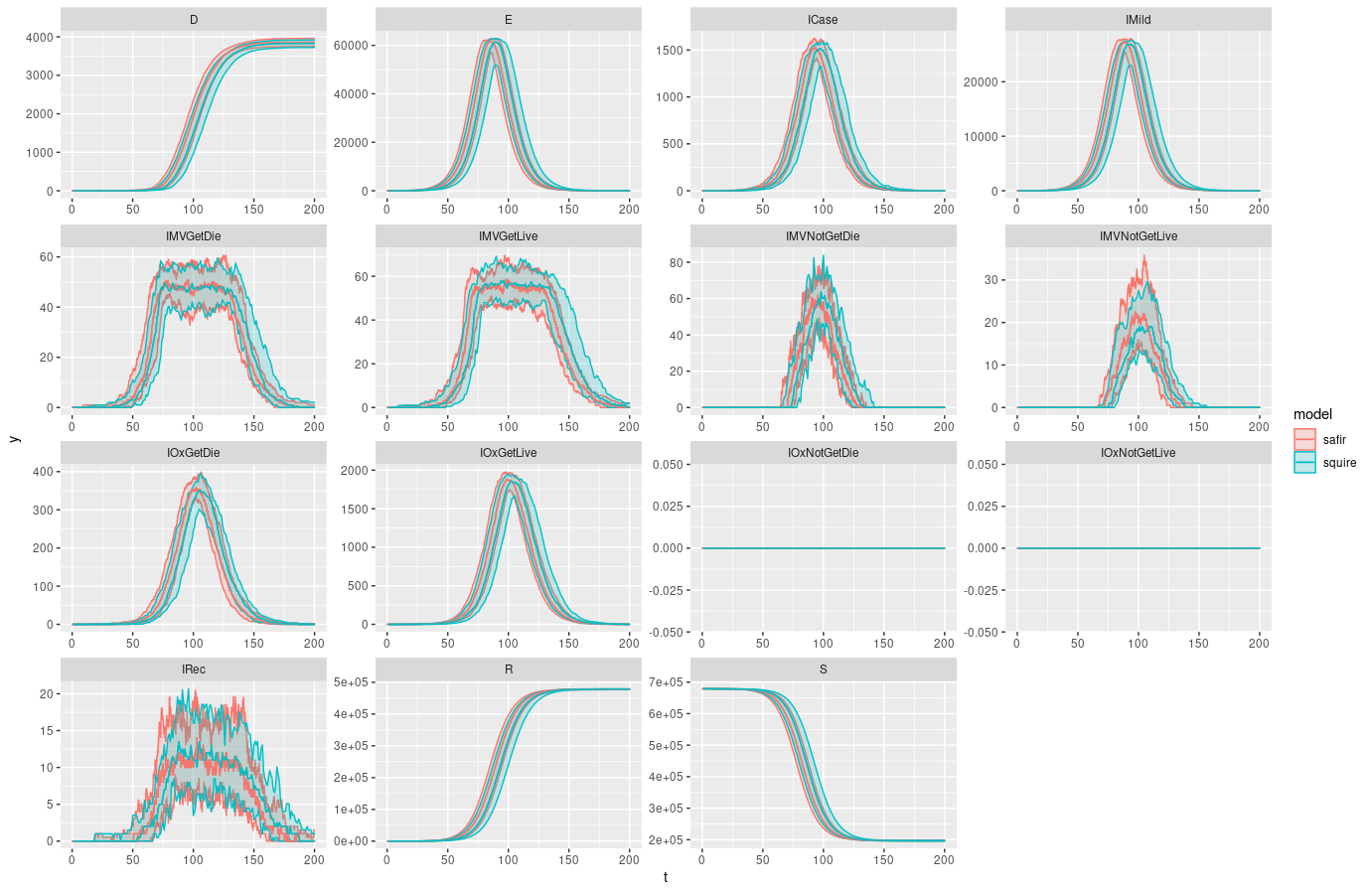
sq_dt <- sq_dt[, .(ymin = quantile(y,0.025), ymax = quantile(y,0.975), y = median(y)), by = .(t,compartment,model)]

Plot Results

It should look nearly identical.

ggplot(data = rbind(saf_dt,sq_dt), aes(t,y,color = model)) +
  geom_line() +
  geom_ribbon(ggplot2::aes(ymin = ymin, ymax = ymax, fill = model), alpha = 0.2) +
  geom_line() +
  facet_wrap(~compartment, scales = "free")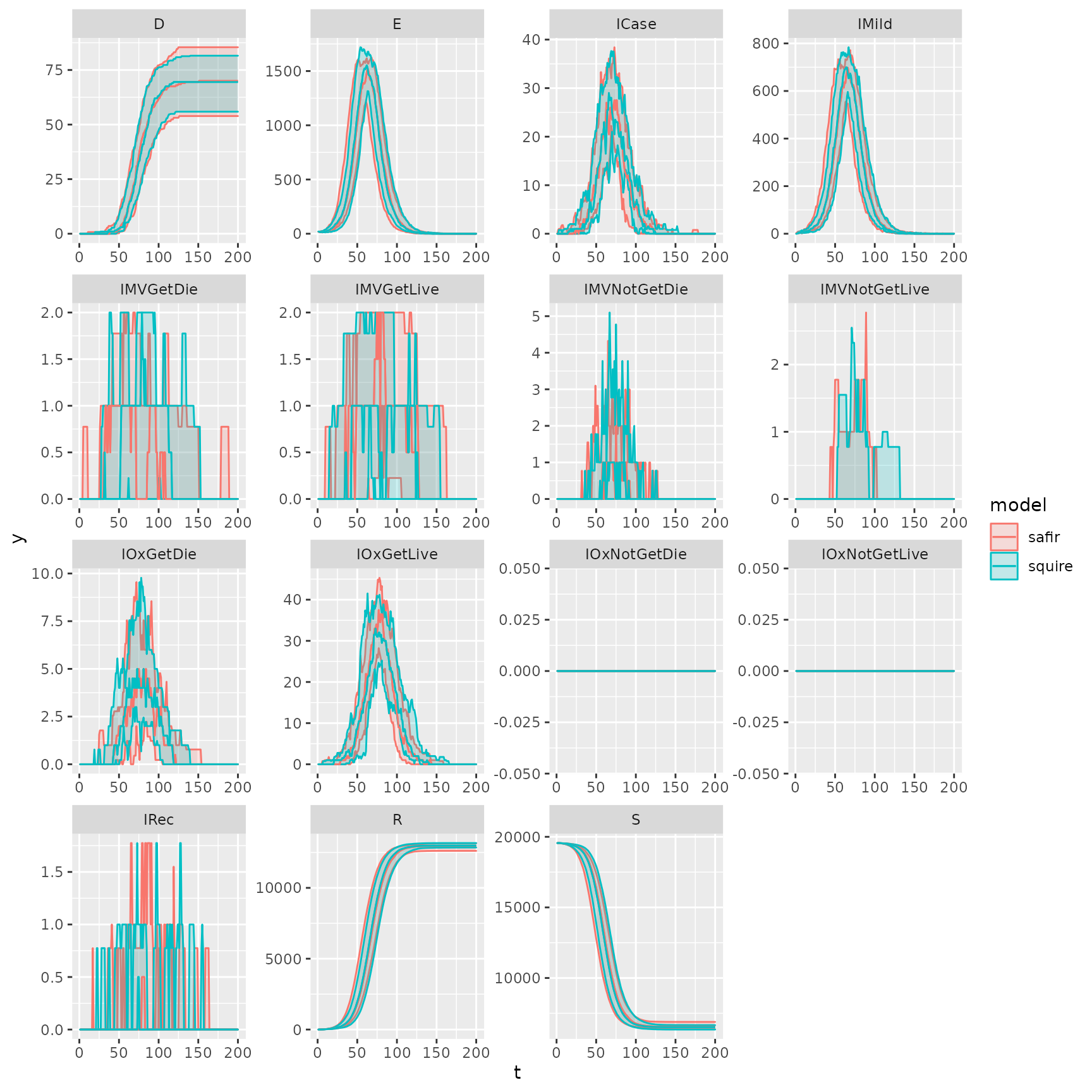

Ensemble plot

Here’s a run of safir vs. squire on GBR with 20 repetitions.

Code design

Parameters

The function get_parameters is used to generate parameters from the squire model, and source code is in R/parameters.R.

Variables

The function create_variables creates state variables for the model. It returns a list containing a individual::CategoricalVariable labeled states which records the disease status of each individual, and a individual::IntegerVariable labeled discrete_age which contains the age bin of each individual.

The main function and code to generate the age variable is found in R/variables.R and the function which generates the disease state variable is found in R/variables_states.R.

Events & Processes

The function create_events creates a list of individual::TargetedEvent object which are responsible for modeling the disease progression of individuals after infection is initiated. attach_event_listeners attaches listeners to each event which execute the state updates and dynamics when each event is triggered for scheduled individuals. Both functions can be found in R/events.R.

setup_events initializes event scheduling based on the initial state of the model. This is needed so that the model can be initialized from any valid state, instead of just S and E persons. It can be found in R/initialize_events.R.

The infection process can either use an R implementation infection_process or C++ implementation infection_process_cpp. The R version is in R/process_infection.R and the C++ one in src/process_infection.cpp.