Working with rminte: R interface for MINTe malaria intervention emulator
Source:vignettes/rminte-tutorial.Rmd
rminte-tutorial.RmdWorking with rminte: R interface for MINTe malaria intervention emulator
This vignette walks through how to:
- Install and load the rminte package
- Run single and multiple scenarios
with
run_minter_scenarios() - Understand the outputs (prevalence, cases, scenario metadata)
- Explore results using tidyverse tools
- Visualize results with ggplot2
- Export results to CSV for further analysis
We treat the ML models as a black box surrogate for
malariasimulation:
- You provide: baseline setting + intervention package(s)
- MINTe returns: predicted prevalence and clinical cases over time
1. Installation and Setup
# Install rminte (if not already installed)
# devtools::install_local("path/to/rminte")

# The Python minte package will be automatically installed via reticulate
# when you first use the package (via py_require)
# Check if minte is available
cat("minte available:", minte_available(), "\n")
#> minte available: TRUE
2. What run_minter_scenarios() does
At a high level, run_minter_scenarios():
- Back-calculates EIR from current prevalence and interventions using the pre-trained estiMINT XGBoost model
- Builds a scenario table with baseline EIR, current and future ITN/IRS/LSM, vector behaviour, resistance & net quality
- Runs the neural emulator to predict:
- Under-5 daily prevalence trajectories
- All-age daily clinical incidence trajectories per 1000
- Returns a results object with:
-
prevalence- Data frame of prevalence over time for each scenario -
cases- Data frame of clinical cases over time for each scenario -
scenario_meta- Per-scenario metadata including EIR validity -
eir_valid- TRUE/FALSE flag -
benchmarks- Runtime timings (optional)
-
3. A Single Simple Scenario
Here we run one scenario by passing single values (or length-1 vectors).
# Example: a single scenario
res_one <- run_minter_scenarios(
 scenario_tag = "example_scenario",
 res_use = 0.2,        # current resistance
 py_only = 0.3,        # pyrethroid-only net coverage
 py_pbo = 0.2,         # PBO net coverage
 py_pyrrole = 0.1,     # pyrrole net coverage
 py_ppf = 0.05,        # PPF net coverage
 prev = 0.55,          # current under-5 prevalence at decision time
 Q0 = 0.92,            # proportion of bites indoors
 phi = 0.85,           # proportion of bites while people are in bed
 season = 0,           # 0 = perennial, 1 = strongly seasonal
 irs = 0.4,            # current IRS coverage
 irs_future = 0.4,     # future IRS coverage
 lsm = 0.2,            # future LSM coverage
 routine = 1,          # 1 = routine ITN distribution on
 itn_future = 0.45,    # future ITN coverage
 net_type_future = "py_only"
)

# Print summary
print(res_one)
#> MINTer Results
#> ==============
#> Prevalence predictions: 156 rows
#> Cases predictions: 156 rows
#> Scenarios: 1
#> EIR valid: TRUE
4. Understanding the Output Structure
The result object exposes the main outputs as list elements:
-
res_one$prevalence- Data frame with prevalence over time -
res_one$cases- Data frame with clinical cases over time
# View first few rows of prevalence
cat("Prevalence (head):\n")
#> Prevalence (head):
head(res_one$prevalence)
#>   index timestep prevalence model_type         scenario     scenario_tag
#> 1     0        1  0.5459521       LSTM example_scenario example_scenario
#> 2     0        2  0.5551386       LSTM example_scenario example_scenario
#> 3     0        3  0.5465310       LSTM example_scenario example_scenario
#> 4     0        4  0.5329272       LSTM example_scenario example_scenario
#> 5     0        5  0.5144109       LSTM example_scenario example_scenario
#> 6     0        6  0.4937868       LSTM example_scenario example_scenario
#>   eir_valid
#> 1      TRUE
#> 2      TRUE
#> 3      TRUE
#> 4      TRUE
#> 5      TRUE
#> 6      TRUE
# View first few rows of cases
cat("\nCases (head):\n")
#>
#> Cases (head):
head(res_one$cases)
#>   index timestep     cases model_type         scenario     scenario_tag
#> 1     0        1 2.5116408       LSTM example_scenario example_scenario
#> 2     0        2 1.5747907       LSTM example_scenario example_scenario
#> 3     0        3 0.7914336       LSTM example_scenario example_scenario
#> 4     0        4 0.5347684       LSTM example_scenario example_scenario
#> 5     0        5 0.4381712       LSTM example_scenario example_scenario
#> 6     0        6 0.3793794       LSTM example_scenario example_scenario
#>   eir_valid
#> 1      TRUE
#> 2      TRUE
#> 3      TRUE
#> 4      TRUE
#> 5      TRUE
#> 6 TRUE5. Running Multiple Scenarios
Now let’s compare several intervention strategies. We’ll create scenarios for:
- No intervention (baseline)
- IRS only
- LSM only
- Different net types (py_only, py_pbo, py_pyrrole, py_ppf)
- Combinations with LSM
# Define multiple scenarios
scenarios <- list(
 list(tag = "no_intervention", irs = 0.0, irs_future = 0.0, lsm = 0.0,
      py_only = 0.3, py_pbo = 0.2, py_pyrrole = 0.1, py_ppf = 0.05),
 list(tag = "irs_only", irs = 0.5, irs_future = 0.5, lsm = 0.0,
      py_only = 0.3, py_pbo = 0.2, py_pyrrole = 0.1, py_ppf = 0.05),
 list(tag = "lsm_only", irs = 0.0, irs_future = 0.0, lsm = 0.3,
      py_only = 0.3, py_pbo = 0.2, py_pyrrole = 0.1, py_ppf = 0.05),
 list(tag = "py_only_only", irs = 0.0, irs_future = 0.0, lsm = 0.0,
      py_only = 0.5, py_pbo = 0.0, py_pyrrole = 0.0, py_ppf = 0.0),
 list(tag = "py_only_with_lsm", irs = 0.0, irs_future = 0.0, lsm = 0.3,
      py_only = 0.5, py_pbo = 0.0, py_pyrrole = 0.0, py_ppf = 0.0),
 list(tag = "py_pbo_only", irs = 0.0, irs_future = 0.0, lsm = 0.0,
      py_only = 0.0, py_pbo = 0.5, py_pyrrole = 0.0, py_ppf = 0.0),
 list(tag = "py_pbo_with_lsm", irs = 0.0, irs_future = 0.0, lsm = 0.3,
      py_only = 0.0, py_pbo = 0.5, py_pyrrole = 0.0, py_ppf = 0.0),
 list(tag = "py_ppf_only", irs = 0.0, irs_future = 0.0, lsm = 0.0,
      py_only = 0.0, py_pbo = 0.0, py_pyrrole = 0.0, py_ppf = 0.5),
 list(tag = "py_ppf_with_lsm", irs = 0.0, irs_future = 0.0, lsm = 0.3,
      py_only = 0.0, py_pbo = 0.0, py_pyrrole = 0.0, py_ppf = 0.5),
 list(tag = "py_pyrrole_only", irs = 0.0, irs_future = 0.0, lsm = 0.0,
      py_only = 0.0, py_pbo = 0.0, py_pyrrole = 0.5, py_ppf = 0.0),
 list(tag = "py_pyrrole_with_lsm", irs = 0.0, irs_future = 0.0, lsm = 0.3,
      py_only = 0.0, py_pbo = 0.0, py_pyrrole = 0.5, py_ppf = 0.0)
)

n <- length(scenarios)

# Extract vectors for each parameter
res_multi <- run_minter_scenarios(
 scenario_tag = sapply(scenarios, `[[`, "tag"),
 res_use = rep(0.2, n),
 py_only = sapply(scenarios, `[[`, "py_only"),
 py_pbo = sapply(scenarios, `[[`, "py_pbo"),
 py_pyrrole = sapply(scenarios, `[[`, "py_pyrrole"),
 py_ppf = sapply(scenarios, `[[`, "py_ppf"),
 prev = rep(0.55, n),
 Q0 = rep(0.92, n),
 phi = rep(0.85, n),
 season = rep(0, n),
 irs = sapply(scenarios, `[[`, "irs"),
 irs_future = sapply(scenarios, `[[`, "irs_future"),
 lsm = sapply(scenarios, `[[`, "lsm"),
 routine = rep(1, n),
 benchmark = TRUE
)
#>
#> === Benchmark Results ===
#> Pre-load models to cache: 0.000 seconds
#> Run EIR predictions (11 scenarios): 0.054 seconds
#> Run Prevalence NN (11 scenarios): 0.043 seconds
#> Run Cases NN (11 scenarios): 0.059 seconds
#>
#> Total time: 0.157 seconds
#> ==============================

print(res_multi)
#> MINTer Results
#> ==============
#> Prevalence predictions: 1716 rows
#> Cases predictions: 1716 rows
#> Scenarios: 11
#> EIR valid: TRUE
#>
#> Benchmarks:
#>    preload_models : 3.099442e-06
#>    run_eir_models : 0.05415201
#>    run_neural_network_prevalence : 0.04301357
#>    run_neural_network_cases : 0.05899692
#>    total : 0.1569171
#>    total_scenarios : 11
6. Exploring Results with dplyr
Let’s use tidyverse tools to analyze the results.
# First few rows by scenario
res_multi$prevalence %>%
 group_by(scenario_tag) %>%
 slice_head(n = 3) %>%
 print(n = 20)
#> # A tibble: 33 × 7
#> # Groups:   scenario_tag [11]
#>    index timestep prevalence model_type scenario         scenario_tag  eir_valid
#>    <dbl>    <dbl>      <dbl> <chr>      <chr>            <chr>         <lgl>
#>  1     1        1      0.516 LSTM       irs_only         irs_only      FALSE
#>  2     1        2      0.522 LSTM       irs_only         irs_only      FALSE
#>  3     1        3      0.511 LSTM       irs_only         irs_only      FALSE
#>  4     2        1      0.459 LSTM       lsm_only         lsm_only      TRUE
#>  5     2        2      0.499 LSTM       lsm_only         lsm_only      TRUE
#>  6     2        3      0.499 LSTM       lsm_only         lsm_only      TRUE
#>  7     0        1      0.459 LSTM       no_intervention  no_intervent… TRUE
#>  8     0        2      0.499 LSTM       no_intervention  no_intervent… TRUE
#>  9     0        3      0.499 LSTM       no_intervention  no_intervent… TRUE
#> 10     3        1      0.486 LSTM       py_only_only     py_only_only  TRUE
#> 11     3        2      0.540 LSTM       py_only_only     py_only_only  TRUE
#> 12     3        3      0.541 LSTM       py_only_only     py_only_only  TRUE
#> 13     4        1      0.486 LSTM       py_only_with_lsm py_only_with… TRUE
#> 14     4        2      0.540 LSTM       py_only_with_lsm py_only_with… TRUE
#> 15     4        3      0.541 LSTM       py_only_with_lsm py_only_with… TRUE
#> 16     5        1      0.475 LSTM       py_pbo_only      py_pbo_only   TRUE
#> 17     5        2      0.518 LSTM       py_pbo_only      py_pbo_only   TRUE
#> 18     5        3      0.520 LSTM       py_pbo_only      py_pbo_only   TRUE
#> 19     6        1      0.475 LSTM       py_pbo_with_lsm  py_pbo_with_… TRUE
#> 20     6        2      0.518 LSTM       py_pbo_with_lsm  py_pbo_with_… TRUE
#> # ℹ 13 more rows
# Mean prevalence over all timesteps by scenario
mean_prev <- res_multi$prevalence %>%
 group_by(scenario_tag) %>%
 summarise(mean_prevalence = mean(prevalence, na.rm = TRUE)) %>%
 arrange(mean_prevalence)

cat("\nMean prevalence by scenario (sorted):\n")
#>
#> Mean prevalence by scenario (sorted):
print(mean_prev)
#> # A tibble: 11 × 2
#>    scenario_tag        mean_prevalence
#>    <chr>                         <dbl>
#>  1 irs_only                      0.456
#>  2 lsm_only                      0.481
#>  3 py_ppf_with_lsm               0.494
#>  4 py_pbo_with_lsm               0.505
#>  5 py_pyrrole_with_lsm           0.509
#>  6 no_intervention               0.511
#>  7 py_only_with_lsm              0.522
#>  8 py_ppf_only                   0.529
#>  9 py_pbo_only                   0.534
#> 10 py_pyrrole_only               0.537
#> 11 py_only_only                  0.553
# Mean cases by scenario
mean_cases <- res_multi$cases %>%
 group_by(scenario_tag) %>%
 summarise(mean_cases = mean(cases, na.rm = TRUE)) %>%
 arrange(mean_cases)

cat("\nMean cases by scenario (sorted):\n")
#>
#> Mean cases by scenario (sorted):
print(mean_cases)
#> # A tibble: 11 × 2
#>    scenario_tag        mean_cases
#>    <chr>                    <dbl>
#>  1 irs_only                  1.52
#>  2 py_ppf_with_lsm           1.68
#>  3 lsm_only                  1.73
#>  4 py_pbo_with_lsm           1.77
#>  5 py_pyrrole_with_lsm       1.77
#>  6 py_only_with_lsm          1.79
#>  7 py_ppf_only               1.90
#>  8 no_intervention           1.92
#>  9 py_pyrrole_only           1.95
#> 10 py_pbo_only               1.95
#> 11 py_only_only              1.98
7. Visualization with ggplot2
Prevalence Over Time (All Scenarios)
ggplot(res_multi$prevalence, aes(x = timestep, y = prevalence,
                                  color = scenario_tag)) +
 geom_line(linewidth = 0.8, alpha = 0.8) +
 labs(
   title = "Malaria Prevalence Over Time by Intervention Strategy",
   subtitle = "Under-5 prevalence predicted by MINTe neural emulator",
   x = "Timestep (14-day periods)",
   y = "Prevalence",
   color = "Scenario"
 ) +
 theme_minimal() +
 theme(legend.position = "right") +
 scale_color_viridis_d()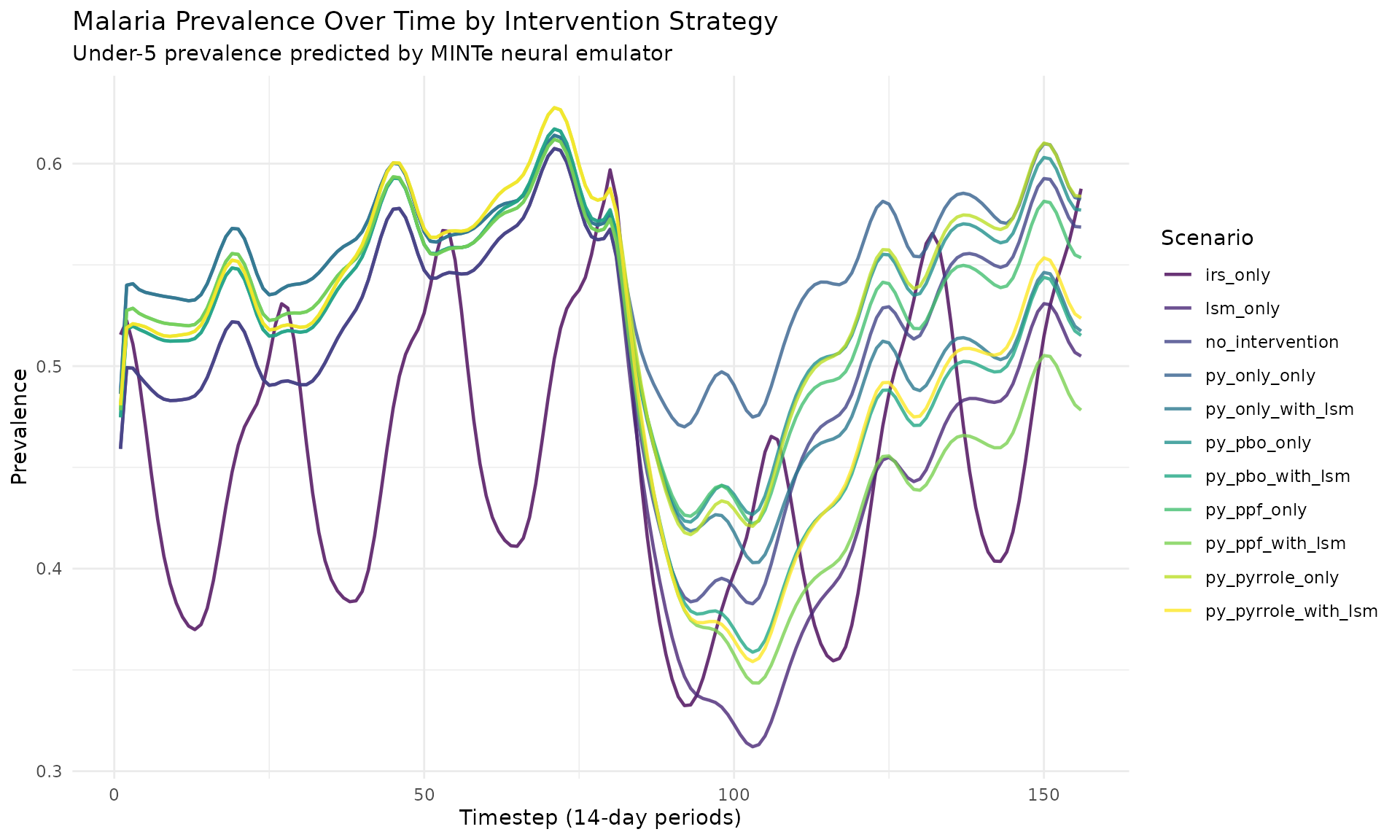
Cases Over Time (All Scenarios)
ggplot(res_multi$cases, aes(x = timestep, y = cases,
                             color = scenario_tag)) +
 geom_line(linewidth = 0.8, alpha = 0.8) +
 labs(
   title = "Clinical Cases Over Time by Intervention Strategy",
   subtitle = "Cases per 1000 predicted by MINTe neural emulator",
   x = "Timestep (14-day periods)",
   y = "Clinical Cases (per 1000)",
   color = "Scenario"
 ) +
 theme_minimal() +
 theme(legend.position = "right") +
 scale_color_viridis_d()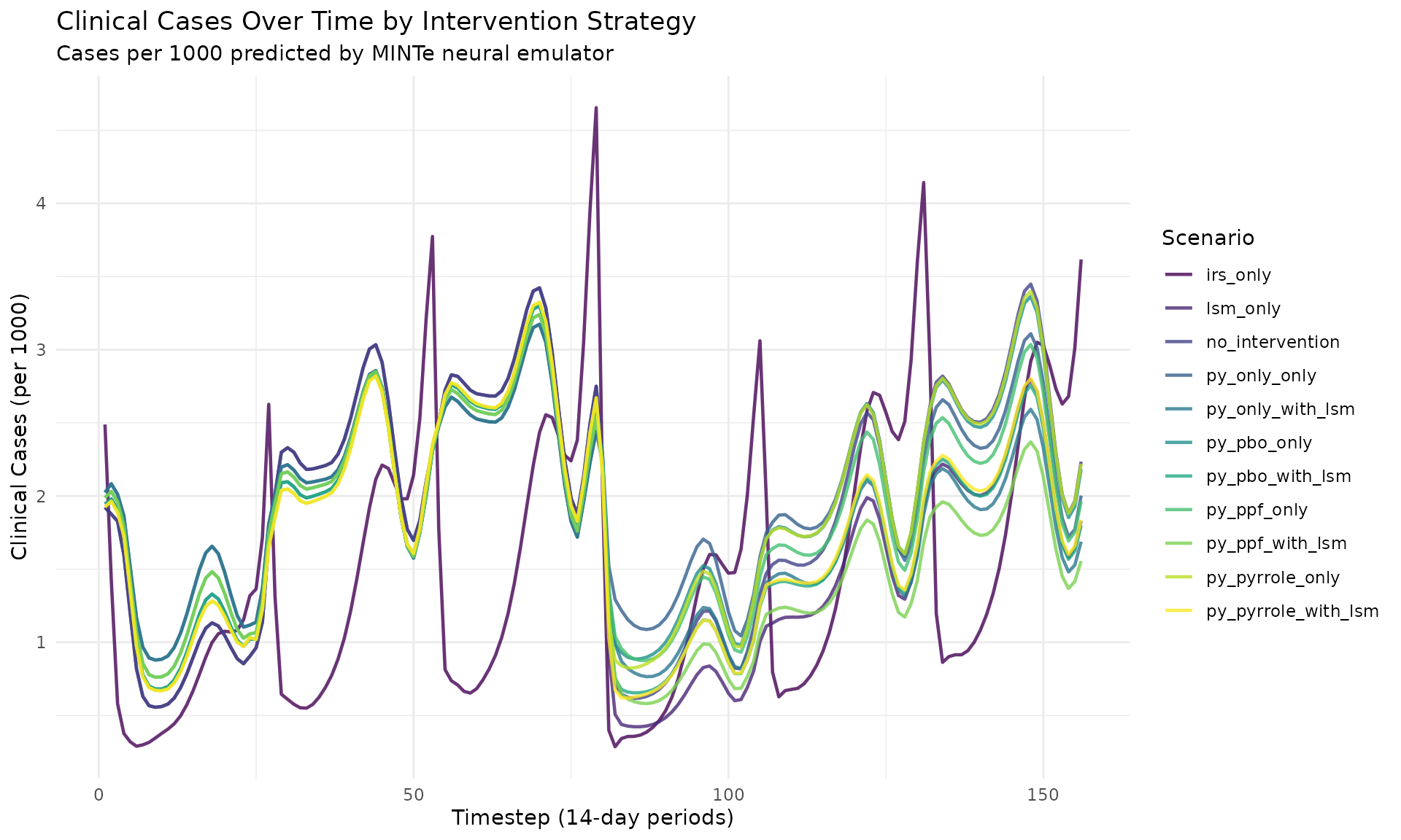
Comparing Selected Scenarios
# Compare key scenarios
selected <- c("no_intervention", "irs_only", "py_pbo_only", "py_pyrrole_with_lsm")

res_multi$prevalence %>%
 filter(scenario_tag %in% selected) %>%
 ggplot(aes(x = timestep, y = prevalence, color = scenario_tag)) +
 geom_line(linewidth = 1.2) +
 labs(
   title = "Comparing Key Intervention Strategies",
   x = "Timestep (14-day periods)",
   y = "Prevalence",
   color = "Scenario"
 ) +
 theme_minimal() +
 theme(legend.position = "bottom") +
 scale_color_brewer(palette = "Set1")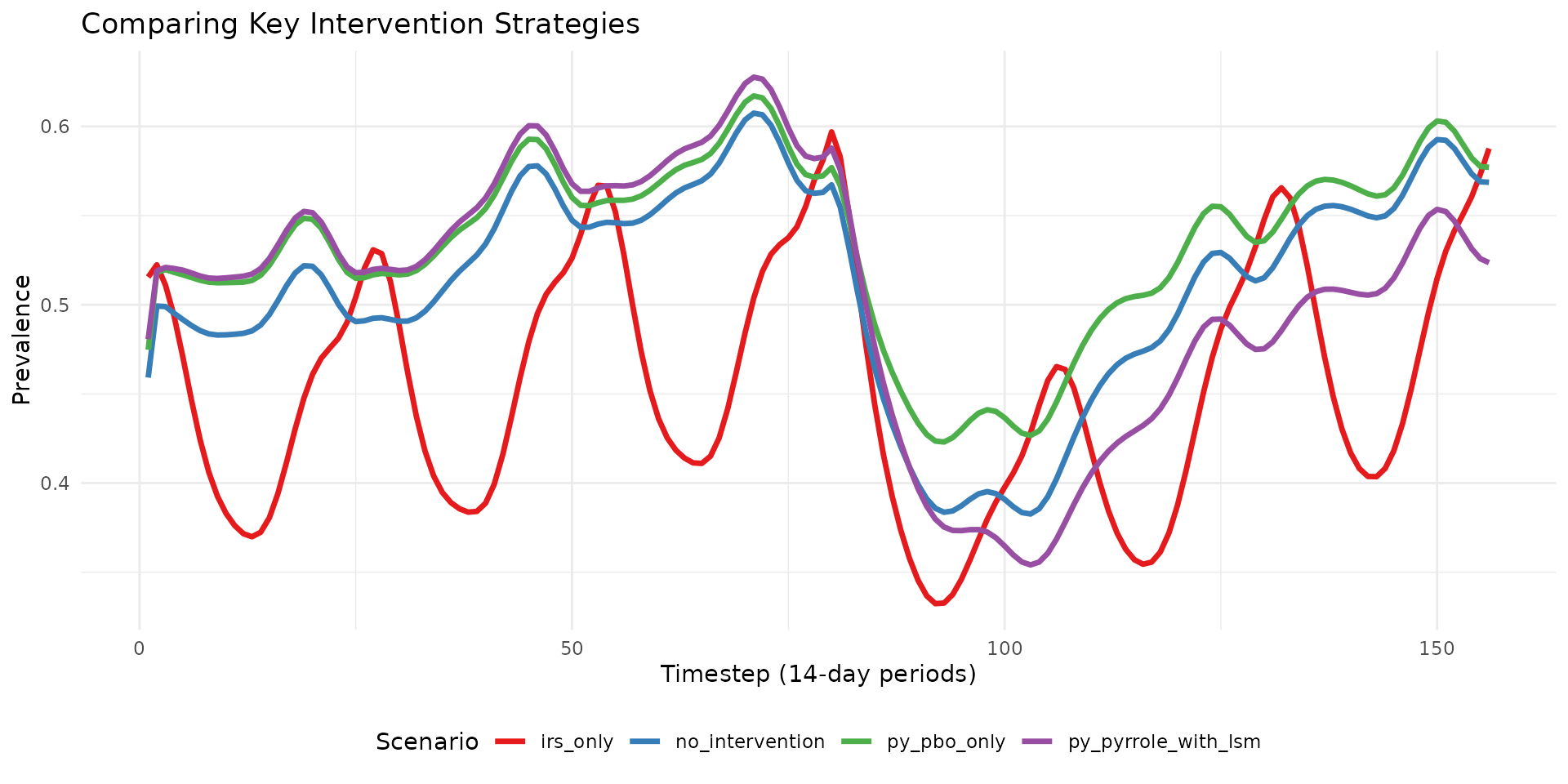
Bar Chart of Mean Prevalence
mean_prev %>%
 mutate(scenario_tag = reorder(scenario_tag, mean_prevalence)) %>%
 ggplot(aes(x = scenario_tag, y = mean_prevalence, fill = scenario_tag)) +
 geom_col() +
 coord_flip() +
 labs(
   title = "Mean Prevalence by Intervention Strategy",
   x = "Scenario",
   y = "Mean Prevalence"
 ) +
 theme_minimal() +
 theme(legend.position = "none") +
 scale_fill_viridis_d()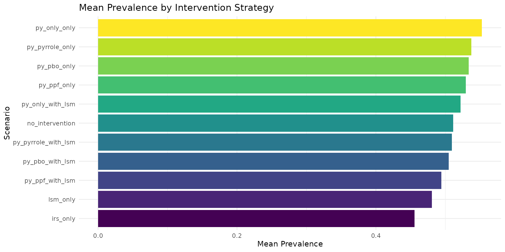
8. Using Built-in Plotting Functions
rminte also provides convenience plotting functions:
# Using the built-in plot_prevalence function
plot_prevalence(res_multi, title = "Prevalence Trajectories")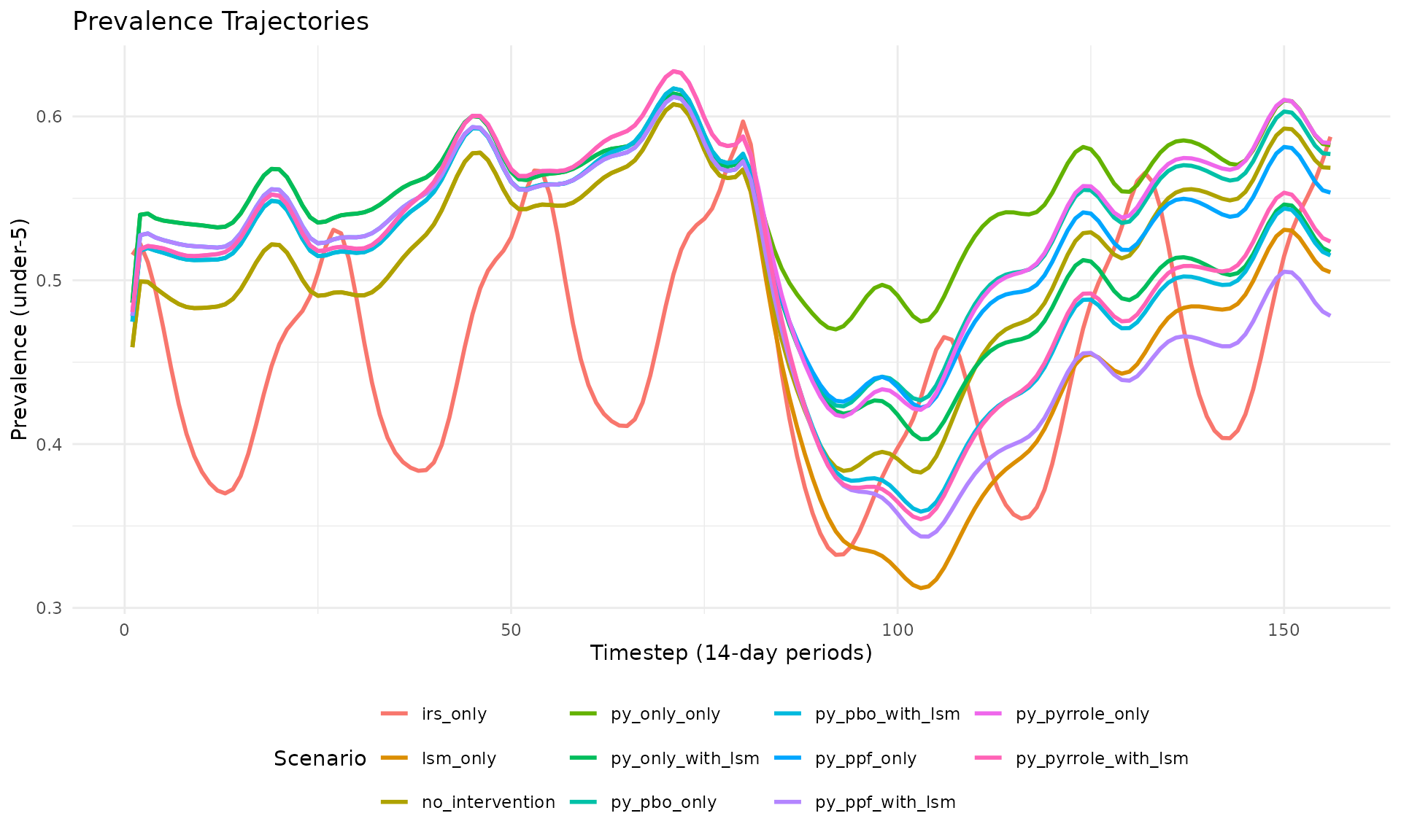
# Using the built-in plot_cases function
plot_cases(res_multi, title = "Cases Trajectories")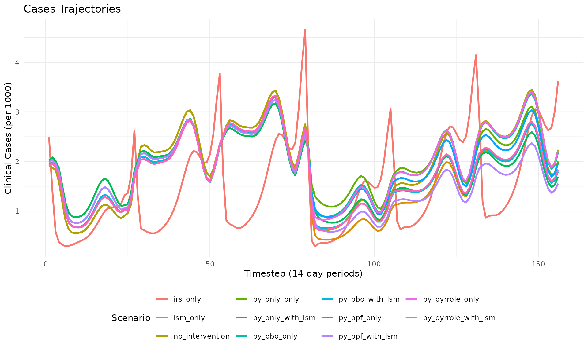
10. Utility Functions
rminte provides several utility functions:
# Calculate net effectiveness from resistance
dn0_result <- calculate_overall_dn0(
 resistance_level = 0.3,
 py_only = 0.4,
 py_pbo = 0.3,
 py_pyrrole = 0.2,
 py_ppf = 0.1
)
cat("Calculated dn0:", dn0_result$dn0, "\n")
#> Calculated dn0: 0.4193867
cat("Total ITN use:", dn0_result$itn_use, "\n")
#> Total ITN use: 1

# Get available net types
net_types <- available_net_types()
cat("Available net types:", paste(net_types, collapse = ", "), "\n")
#> Available net types: pyrethroid_only, pyrethroid_pbo, pyrethroid_ppf, pyrethroid_pyrrole
Summary
This vignette demonstrated how to:
-
Run scenarios using
run_minter_scenarios()with various intervention parameters -
Access results via the returned list
(
$prevalence,$cases,$scenario_meta) - Analyze data using dplyr for grouping and summarizing
- Visualize with ggplot2 or built-in plotting functions
- Export results to CSV for further analysis
The rminte package provides a seamless R interface to the Python MINTe neural emulator, allowing you to rapidly evaluate malaria intervention strategies without running full simulations.
Session Info
sessionInfo()
#> R version 4.5.2 (2025-10-31)
#> Platform: x86_64-pc-linux-gnu
#> Running under: Ubuntu 24.04.3 LTS
#>
#> Matrix products: default
#> BLAS:   /usr/lib/x86_64-linux-gnu/openblas-pthread/libblas.so.3
#> LAPACK: /usr/lib/x86_64-linux-gnu/openblas-pthread/libopenblasp-r0.3.26.so;  LAPACK version 3.12.0
#>
#> locale:
#>  [1] LC_CTYPE=C.UTF-8       LC_NUMERIC=C           LC_TIME=C.UTF-8
#>  [4] LC_COLLATE=C.UTF-8     LC_MONETARY=C.UTF-8    LC_MESSAGES=C.UTF-8
#>  [7] LC_PAPER=C.UTF-8       LC_NAME=C              LC_ADDRESS=C
#> [10] LC_TELEPHONE=C         LC_MEASUREMENT=C.UTF-8 LC_IDENTIFICATION=C
#>
#> time zone: UTC
#> tzcode source: system (glibc)
#>
#> attached base packages:
#> [1] stats     graphics  grDevices utils     datasets  methods   base
#>
#> other attached packages:
#> [1] tidyr_1.3.1   ggplot2_4.0.1 dplyr_1.1.4   rminte_0.1.0
#>
#> loaded via a namespace (and not attached):
#>  [1] Matrix_1.7-4       gtable_0.3.6       jsonlite_2.0.0     compiler_4.5.2
#>  [5] tidyselect_1.2.1   Rcpp_1.1.0         jquerylib_0.1.4    systemfonts_1.3.1
#>  [9] scales_1.4.0       textshaping_1.0.4  png_0.1-8          yaml_2.3.11
#> [13] fastmap_1.2.0      here_1.0.2         reticulate_1.44.1  lattice_0.22-7
#> [17] R6_2.6.1           labeling_0.4.3     generics_0.1.4     knitr_1.50
#> [21] tibble_3.3.0       desc_1.4.3         rprojroot_2.1.1    RColorBrewer_1.1-3
#> [25] bslib_0.9.0        pillar_1.11.1      rlang_1.1.6        utf8_1.2.6
#> [29] cachem_1.1.0       xfun_0.54          S7_0.2.1           fs_1.6.6
#> [33] sass_0.4.10        viridisLite_0.4.2  cli_3.6.5          withr_3.0.2
#> [37] pkgdown_2.2.0      magrittr_2.0.4     digest_0.6.39      grid_4.5.2
#> [41] rappdirs_0.3.3     lifecycle_1.0.4    vctrs_0.6.5        evaluate_1.0.5
#> [45] glue_1.8.0         farver_2.1.2       ragg_1.5.0         purrr_1.2.0
#> [49] rmarkdown_2.30     tools_4.5.2        pkgconfig_2.0.3    htmltools_0.5.9