Tutorial • individual

Introduction

The Susceptible-Infectious-Recovered (SIR) model is the “hello, world!” model for infectious disease simulations, and here we describe how to build it in “individual”. This tutorial will illustrate the use of events, processes, and rendering output.

Specification

To start, we should define some constants. The epidemic will be simulated in a population of 1000, where 5 persons are initially infectious, whose indices are randomly sampled. The effective contact rate $\beta$ will be a function of the deterministic $R_{0}$ and recovery rate $\gamma$ . We also specify dt, which is the size of the time step $(\Delta t)$ . Because individual’s time steps are all of unit length, we scale transition probabilities by dt to create models with different sized steps, interpreting the discrete time model as a discretization of a continuous time model. If the maximum time is tmax then the overall number of time steps is tmax/dt.

N <- 1e3
I0 <- 5
S0 <- N - I0
dt <- 0.1
tmax <- 100
steps <- tmax/dt
gamma <- 1/10
R0 <- 2.5
beta <- R0 * gamma
health_states <- c("S","I","R")
health_states_t0 <- rep("S",N)
health_states_t0[sample.int(n = N,size = I0)] <- "I"

Next, we will define the individual::CategoricalVariable which should store the model’s “state”.

health <- CategoricalVariable$new(categories = health_states,initial_values = health_states_t0)

Processes

In order to model infection, we need a process. This is a function that takes only a single argument, t, for the current time step (unused here, but can model time-dependent processes, such as seasonality or school holiday). Within the function, we get the current number of infectious individuals, then calculate the per-capita force of infection on each susceptible person, $\lambda = \beta I/N$ . Next we get a individual::Bitset containing those susceptible individuals and use the sample method to randomly select those who will be infected on this time step. The probability is given by $1 - e^{-\lambda\Delta t}$ . This is the same as the CDF of an exponential random variate so we use stats::pexp to compute that quantity. Finally, we queue a state update for those individuals who were sampled.

infection_process <- function(t){
  I <- health$get_size_of("I")
  foi <- beta * I/N
  S <- health$get_index_of("S")
  S$sample(rate = pexp(q = foi * dt))
  health$queue_update(value = "I",index = S)
}

Events

Now we need to model recovery. For geometrically distributed infectious periods, we could use another process that randomly samples some individuals each time step to recover, but we’ll use a individual::TargetedEvent to illustrate their use. The recovery event is quite simple, and the “listener” which is added is a function that is called when the event triggers, taking target, a individual::Bitset of scheduled individuals, as its second argument. Those individuals are scheduled for a state update within the listener function body.

recovery_event <- TargetedEvent$new(population_size = N)
recovery_event$add_listener(function(t, target) {
  health$queue_update("R", target)
})

Finally, we need to define a recovery process that queues future recovery events. We first get individual::Bitset objects of those currently infectious individuals and those who have already been scheduled for a recovery. Then, using bitwise operations, we get the intersection of already infectious persons with persons who have not been scheduled, precisely those who need to have recovery times sampled and recoveries scheduled. We sample those times from stats::rgeom, where the probability for recovery is $1-e^{-\gamma \Delta t}$ . Note that we add one to the resulting vector, because by default R uses a “number of failures” parameterization rather than “number of trials”, meaning it would be possible for an individual to be infectious for 0 time steps without the correction. Finally we schedule the recovery using the recovery event object.

We note at this point would be possible to queue the recovery event at the same time the infection state update was made, but we separate event and process for illustration of how the package works.

recovery_process <- function(t){
  I <- health$get_index_of("I")
  already_scheduled <- recovery_event$get_scheduled()
  I$and(already_scheduled$not(inplace = TRUE))
  rec_times <- rgeom(n = I$size(),prob = pexp(q = gamma * dt)) + 1
  recovery_event$schedule(target = I,delay = rec_times)
}

Rendering

The last thing to do before simulating the model is rendering output to plot. We use a individual::Render object which stores output from the model, which is tracked each time step. To do so requires another process, for which we use the “prefab” individual::categorical_count_renderer_process.

health_render <- Render$new(timesteps = steps)
health_render_process <- categorical_count_renderer_process(
  renderer = health_render,
  variable = health,
  categories = health_states
)

Simulation

Finally, the simulation can be run by passing objects to the individual::simulation_loop function:

simulation_loop(
  variables = list(health),
  events = list(recovery_event),
  processes = list(infection_process,recovery_process,health_render_process),
  timesteps = steps
)

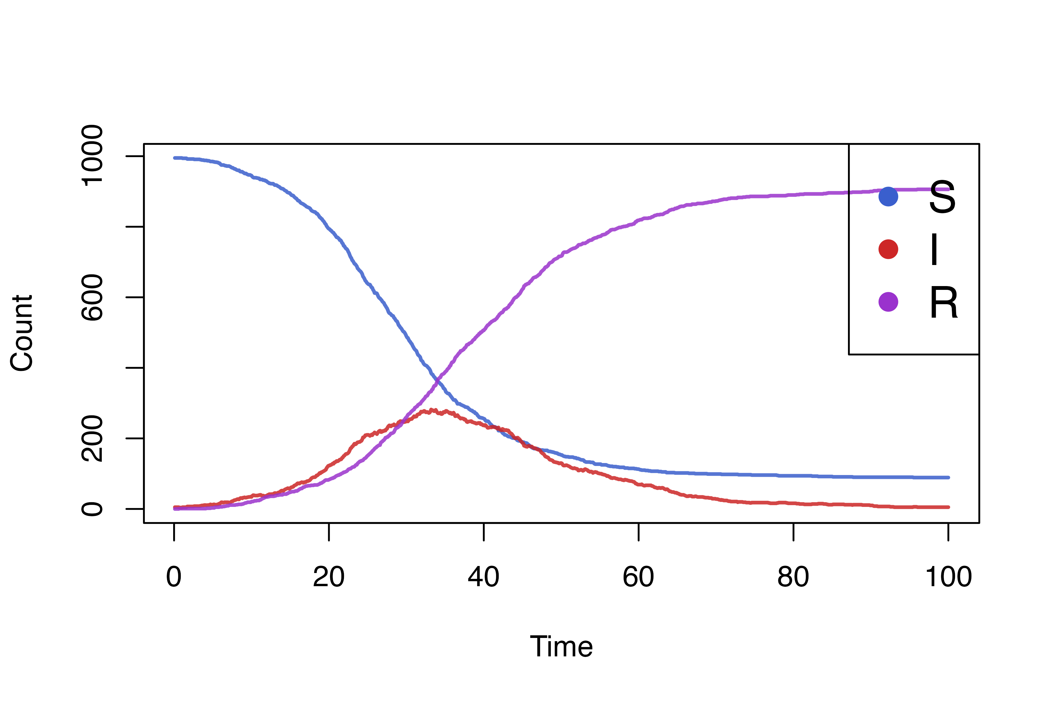
We can easily plot the results by accessing the renderer.

states <- health_render$to_dataframe()
health_cols <-  c("royalblue3","firebrick3","darkorchid3")
matplot(
  x = states[[1]]*dt, y = states[-1],
  type="l",lwd=2,lty = 1,col = adjustcolor(col = health_cols, alpha.f = 0.85),
  xlab = "Time",ylab = "Count"
)
legend(
  x = "topright",pch = rep(16,3),
  col = health_cols,bg = "transparent",
  legend = health_states, cex = 1.5
)