Version 0.1
The R package covfefe performs Computational Validation For Estimating Falciparum Epidemiology (ahem). More specifically, it provides a flexible framework for simulating genetic data from P. falciparum transmission models.
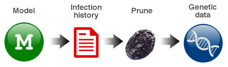
We start with data on infection histories - i.e. who became infected when, who did this infection originate from, when did this episode recover, etc. We then specify a subset of samples that we are interested in - for example, 100 individuals at day 365. covfefe then prunes the infection history data down to a reduced set that contains only the events that directly impact on the samples that we are interested in. Often the number of sampled hosts is far smaller than the total infected population, or perhaps sampling only occurs at a few time points, meaning the pruned infection history can be much smaller than the complete infection history. Finally, covfefe simulates genetic data from the pruned infection history and from a set of user-defined parameters that specify the genetic model, for example the recombination rate and the number of loci.
By using the infection history as the starting point we ensure that multiple epidemiological models can be plugged into the same tool. Any malaria transmission model that generates infection history data in the format required by covfefe can be used to simulate genetic data, and this format has been designed to be flexible enough to encompass a wide range of models. covfefe also contains it sown simple individual-based model that simulates malaria transmission in multiple demes (partially isolated subpopulations), with or without migration between demes.
This package is still in development, meaning methods are likely to change in the near future. That being said, here are instructions on how to install and run covfefe as it currently stands.
Installation
covfefe relies on the Rcpp package, which requires the following OS-specific steps:
- Windows
- Download and install the appropriate version of Rtools for your version of R. On installation, ensure you check the box to arrange your system PATH as recommended by Rtools
- Mac OS X
- Download and install XCode
- Within XCode go to Preferences : Downloads and install the Command Line Tools
- Linux (Debian/Ubuntu)
-
Install the core software development utilities required for R package development as well as LaTeX by executing
```
sudo apt-get install r-base-dev texlive-full
```
-
Next, ensure that you have devtools installed by running
install.packages("devtools")Finally, install the covfefe package directly from GitHub by running
devtools::install_github("mrc-ide/covfefe")
library(covfefe)
Example analysis
Loading infection history
The analysis pipeline starts by creating a covfefe project. This project will hold all inputs and outputs used by the package, and is a convenient way of keeping everything we need in one place.
myproj <- covfefe_project()Running names(myproj) we can see all the elements that make up a covfefe project, including parameters, distributions, etc. We will talk about each of these elements in due course.
To begin with we need some data on infection histories. For convenience, we will use the in-built individual-based model with default settings, which simulates transmission in a single population.
mysim <- sim_indiv()Again, running names(mysim) we can see the elements that make up mysim, including H - the human population size in each deme, daily_counts - the number of susceptible vs. singly-infected vs. doubly-infected (and so on) individuals on each day, and infection_history - a complete list of critical events. For those who want to understand the infection history format, details can be found here (TODO - link to format).
TODO - demonstrate plotting functions for simulated data.
We continue by loading the infection history into our project.
myproj <- assign_infection_history(myproj, mysim$infection_history)Sampling and pruning
Next, we need to specify how many human hosts we want to sample from, and when. We do this using a simple matrix or data frame with three columns: column 1 gives the time of sampling, column 2 gives the deme that we are sampling from, and column 3 gives the number of hosts to draw at random from the pool of blood-stage individuals at that point in time. Note that in column 3, a value of -1 indicates that all blood stage hosts should be sampled. In this example, we will sample at day 100 and day 365, in a single deme (we only have one deme), and drawing all hosts at the first time point and 100 hosts at the second time point.
mysamp <- data.frame(times = c(100, 365), demes = 1, hosts = c(-1, 100))Next we load this data into our project, taking care to specify the number of demes, which is not always completely obvious from the infection history and sampling data alone.
myproj <- sample_hosts(myproj, mysamp, demes = 1)Finally we prune the infection history down based on the sampling data. Once we have done this, we are free to delete the original infection history data from the project. Doing so will free up space, which might be limited if the infection history data is very large, but will also mean we cannot re-run sample_hosts without first re-loading the infection history data.
myproj <- prune(myproj)
myproj <- delete_infection_history(myproj)
Simulating genetic data
Now that we know which transmission events we are interested in, we can simulate the passing down of genetic information through this infection tree. Two of the most important variables from the genetic point of view are the number of oocysts that develop in the mosquito to produce viable sporozoites, and the number of sporozoites that make it to the liver of a newly infected host to form viable hepatic schizonts. Each of these variables can be specified in terms of a full probability distribution, which is drawn from independently each time a mosquito or human becomes infected.
myproj <- define_oocyst_distribution(myproj, oocysts = dpois(1:10, lambda = 1))
myproj <- define_hepatocyte_distribution(myproj, hepatocytes = dpois(1:10, lambda = 1))
Any distribution can be used, but note that these distributions are assumed to start from 1, as a value of 0 oocysts or 0 hepatic schizonts is impossible given that transmission occured.
Next we must define the loci that we are interested in. We define these in a list of up to 14 elements (one for each chromosome), with each consisting of a vector of genomic positions (in base pairs). In this example our target loci are evenly tiled over chromosomes 1 and 3.
myloci <- list(seq(0, 64e4, 1e4), NULL, seq(0, 100e4, 1e4))Finally we can simulate some genetic data. At this stage we also specify the recombination rate in events per base-pair.
myproj <- sim_genotypes(myproj, myloci, recom_rate = 0.001)Further details of the genetic model can be found here (TODO - link to details of genetic model).
Links
- Download from CRAN at
https://cloud.r-project.org/package=covfefe - Report a bug at
NA
Developers
- Bob Verity
Author, maintainer

