Preparing data and configuration for anatembea • anatembea

Particle Markov chain Monte Carlo (pMCMC) can be computationally expensive. A longer run will not repair invalid counts, incorrectly ordered dates, or a poorly specified initialization. This article therefore prepares and freezes the analysis specification before tuning begins.

At the end of this article you will have:

a checked monthly prevalence dataset;
a documented model specification; and
enough provenance to reproduce the analysis.

The next article, Tuning an anatembea pMCMC, uses that frozen specification to select a particle count and proposal covariance.

Required data

For a single comparison group, run_pmcmc() expects one row per month and at least these columns:

month: a monthly time variable, represented here by zoo::yearmon;
tested: the number of people tested; and
positive: the number who tested positive.

The package includes simulated data that we can use throughout this series.

analysis_data <- dplyr::filter(
  dplyr::select(anatembea::sim_data_tanzania, month, positive, tested),
  month <= zoo::as.yearmon("Dec 2019")
)

head(analysis_data, 4)
#>      month positive tested
#> 1 Jan 2017      204   1000
#> 2 Feb 2017      224   1000
#> 3 Mar 2017      234   1000
#> 4 Apr 2017      256   1000

For paired ANC comparisons such as comparison = "pgmg", prepare separate primigravidae and multigravidae datasets with the same three columns and pass them as data_raw_pg and data_raw_mg. See run_pmcmc() for all supported comparison groups.

Validate before fitting

The helper below checks structural errors while allowing a month in which both counts are missing. anatembea can treat such a month as an unobserved time point, but a missing positive paired with a non-missing tested (or vice versa) is ambiguous and should be resolved.

validate_monthly_prevalence <- function(data) {
  required <- c("month", "positive", "tested")
  missing_columns <- setdiff(required, names(data))
  if (length(missing_columns) > 0) {
    stop("Missing required columns: ", paste(missing_columns, collapse = ", "))
  }

  month_key <- format(data$month, "%Y-%m")
  if (anyNA(month_key)) stop("`month` contains missing or unparseable values.")
  if (is.unsorted(data$month)) stop("Rows must be in chronological order.")
  if (anyDuplicated(month_key)) stop("Each month must appear at most once.")

  one_count_missing <- xor(is.na(data$positive), is.na(data$tested))
  if (any(one_count_missing)) {
    stop("`positive` and `tested` must be missing together.")
  }

  observed <- !is.na(data$positive)
  positive <- data$positive[observed]
  tested <- data$tested[observed]

  if (any(!is.finite(c(positive, tested)))) {
    stop("Observed counts must be finite.")
  }
  if (any(positive != floor(positive) | tested != floor(tested))) {
    stop("Observed counts must be whole numbers.")
  }

  invalid_counts <- positive < 0 | tested < 0 | positive > tested
  if (any(invalid_counts)) {
    stop("Counts must satisfy 0 <= positive <= tested.")
  }

  expected <- format(
    seq(min(data$month), max(data$month), by = 1 / 12),
    "%Y-%m"
  )
  gaps <- setdiff(expected, month_key)
  if (length(gaps) > 0) {
    warning("Missing calendar months: ", paste(gaps, collapse = ", "))
  }

  invisible(data)
}

validate_monthly_prevalence(analysis_data)

invalid_example <- analysis_data[1, ]
invalid_example$positive <- Inf
try(validate_monthly_prevalence(invalid_example))
#> Error in validate_monthly_prevalence(invalid_example) : 
#>   Observed counts must be finite.

invalid_example$positive <- 1.5
try(validate_monthly_prevalence(invalid_example))
#> Error in validate_monthly_prevalence(invalid_example) : 
#>   Observed counts must be whole numbers.

A gap is a month with no row; a missing observation is a row with both counts set to NA. Decide deliberately which representation your analysis uses. Also plot positive / tested and tested over time. Abrupt changes may be real, but they often reveal altered reporting systems, duplicated extracts, or changes in the population being tested.

plot_data <- dplyr::mutate(
  analysis_data,
  prevalence = positive / tested
)

ggplot2::ggplot(plot_data, ggplot2::aes(month, prevalence)) +
  ggplot2::geom_line(colour = "#1F78B4") +
  ggplot2::geom_point(ggplot2::aes(size = tested), alpha = 0.6) +
  ggplot2::scale_y_continuous(limits = c(0, 1)) +
  ggplot2::labs(x = NULL, y = "Observed prevalence", size = "Tested") +
  ggplot2::theme_minimal()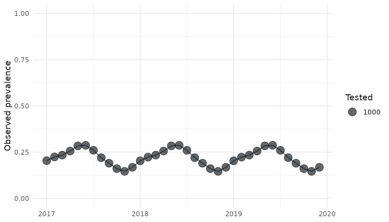

Freeze the scientific specification

Write down the settings that determine what the model means, not just how long it runs. At minimum, record:

comparison and the population represented by each input series;
initial, target_prev, and the initial-condition window;
check_flexibility and start_pf_time;
treatment and seasonality assumptions, including geographic inputs;
fitted parameter names and their order; and
any departure from package defaults.

For example:

analysis_spec <- list(
  analysis_id = "tanzania-u5-example",
  comparison = "u5",
  initial = "fitted",
  check_flexibility = TRUE,
  start_pf_time = 30 * 12,
  prop_treated = 0.4,
  seasonality_on = TRUE,
  fitted_parameters = c("log_init_EIR", "volatility")
)

analysis_spec
#> $analysis_id
#> [1] "tanzania-u5-example"
#> 
#> $comparison
#> [1] "u5"
#> 
#> $initial
#> [1] "fitted"
#> 
#> $check_flexibility
#> [1] TRUE
#> 
#> $start_pf_time
#> [1] 360
#> 
#> $prop_treated
#> [1] 0.4
#> 
#> $seasonality_on
#> [1] TRUE
#> 
#> $fitted_parameters
#> [1] "log_init_EIR" "volatility"

Choose an initialization mode

Use initial = "fitted" when initial transmission intensity should be inferred from the data. In the current implementation, the fitted parameters are ordered as log_init_EIR and then volatility. Proposals for log_init_EIR are bounded between log(1e-3) and log(500) before model evaluation.

Use initial = "informed" when an equilibrium EIR or target prevalence is a scientifically defensible input. Only volatility is then sampled. Because these modes have different parameter spaces, they cannot share a proposal covariance.

Record software, inputs, and seeds

Package behavior can change between releases. Save versions and source revisions alongside every submitted run.

provenance <- list(
  recorded_at = format(Sys.time(), tz = "UTC"),
  R = R.version.string,
  packages = vapply(
    c("anatembea", "mcstate", "dust", "odin.dust", "odin"),
    function(x) as.character(utils::packageVersion(x)),
    character(1)
  ),
  git_commit = tryCatch(
    system2("git", c("rev-parse", "HEAD"), stdout = TRUE, stderr = FALSE),
    error = function(e) NA_character_
  ),
  seeds = c(smoke = 1101L, pilot = 2101L, scale_1 = 3101L)
)

provenance
#> $recorded_at
#> [1] "2026-08-26 08:34:33"
#> 
#> $R
#> [1] "R version 4.6.1 (2026-06-24)"
#> 
#> $packages
#> anatembea   mcstate      dust odin.dust      odin 
#>   "1.1.0"  "0.9.22"  "0.15.3"  "0.3.13"  "1.5.12" 
#> 
#> $git_commit
#> [1] "8e4f3fd7afe16cb5fda63bc7cce215a3ab0dcf7f"
#> 
#> $seeds
#>   smoke   pilot scale_1 
#>    1101    2101    3101

For file-based inputs, tools::md5sum("path/to/input.csv") provides a compact way to detect whether the file has changed. A project-specific library managed with renv can record package versions, but the resolved anatembea commit or release should still be saved explicitly.

Do not install a moving branch such as HEAD in a production job without recording the resolved commit.

Gate: ready to tune?

Proceed only when all of the following are true:

counts, dates, groups, and gaps have been reviewed;
initialization and seasonality return finite, plausible states;
the fitted parameter names and order are recorded;
model assumptions are frozen; and
inputs, software versions, and unique seeds can be reconstructed.

You are now ready to tune the pMCMC.