Plot outputs of estimate_r

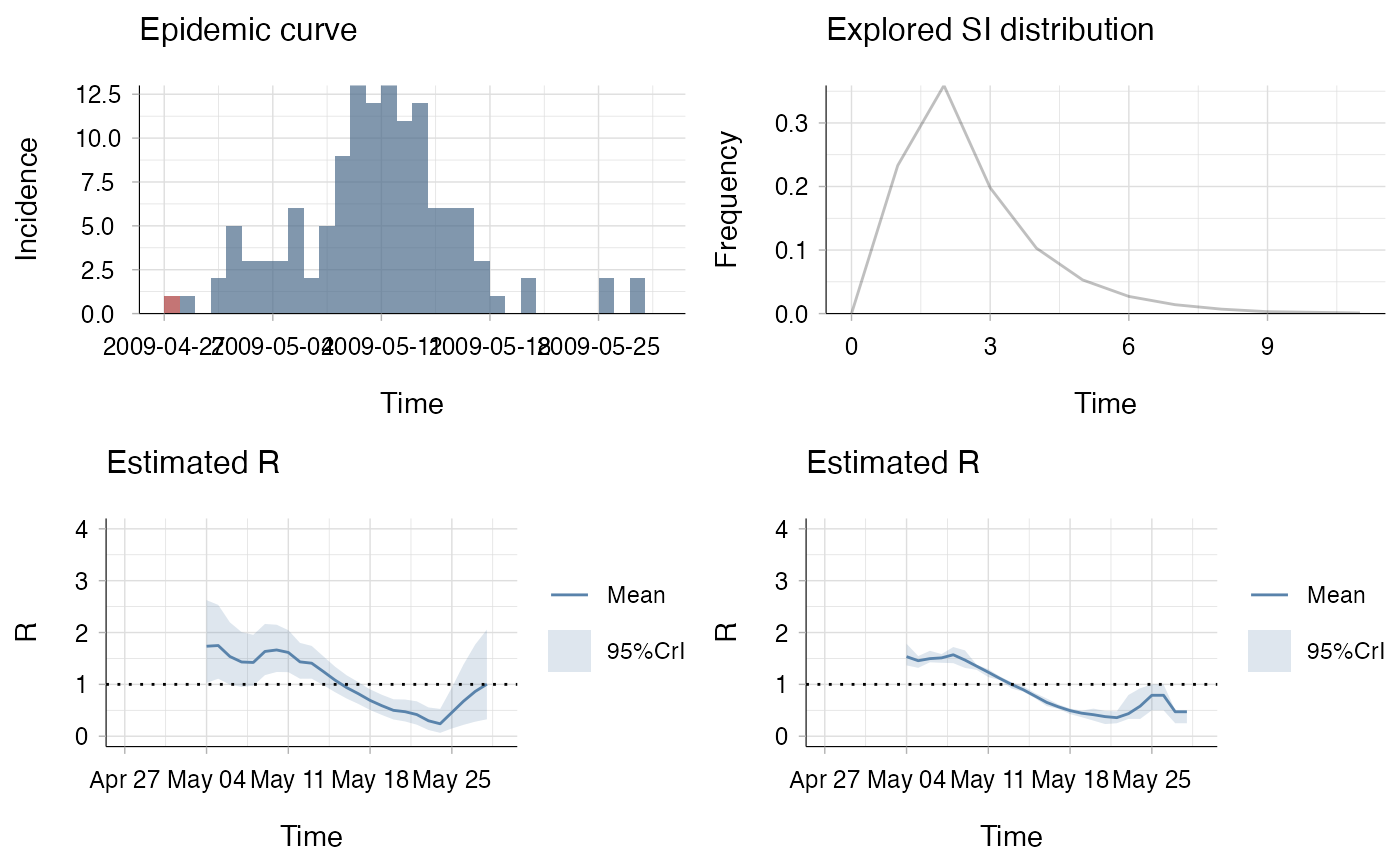
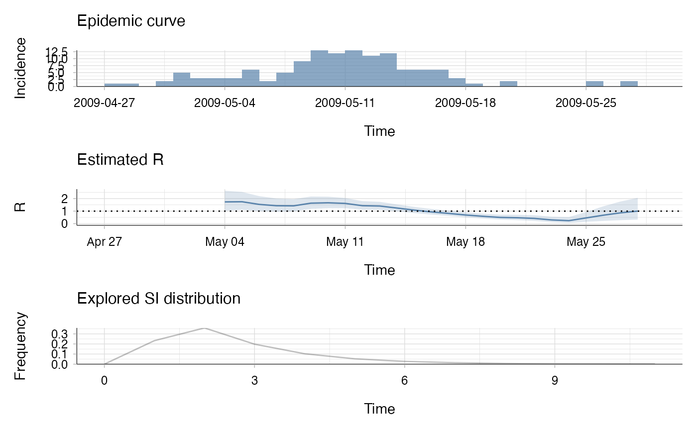
The plot method of estimate_r objects can be used to visualise three types of information. The first one shows the epidemic curve. The second one shows the posterior mean and 95% credible interval of the reproduction number. The estimate for a time window is plotted at the end of the time window. The third plot shows the discrete distribution(s) of the serial interval.

# S3 method for class 'estimate_R'
plot(
  x,
  what = c("all", "incid", "R", "SI"),
  plot_theme = "v2",
  add_imported_cases = FALSE,
  options_I = list(col = palette(), transp = 0.7, xlim = NULL, ylim = NULL, interval =
    1L, xlab = "Time", ylab = "Incidence"),
  options_R = list(col = palette(), transp = 0.2, xlim = NULL, ylim = NULL, xlab =
    "Time", ylab = "R"),
  options_SI = list(prob_min = 0.001, col = "black", transp = 0.25, xlim = NULL, ylim =
    NULL, xlab = "Time", ylab = "Frequency"),
  legend = TRUE,
  ...
)

Arguments

x

The output of function estimate_R or function wallinga_teunis. To plot simultaneous outputs on the same plot use estimate_R_plots function

what

A string specifying what to plot, namely the incidence time series (what='incid'), the estimated reproduction number (what='R'), the serial interval distribution (what='SI', or all three (what='all')).

plot_theme

A string specifying whether to use the original plot theme (plot_theme = "original") or an alternative plot theme (plot_theme = "v2"). The plot_theme is "v2" by default.

add_imported_cases

A boolean to specify whether, on the incidence time series plot, to add the incidence of imported cases.

options_I

For what = "incid" or "all". A list of graphical options:

col: A color or vector of colors used for plotting incid. By default uses the default R colors.
transp: A numeric value between 0 and 1 used to monitor transparency of the bars plotted. Defaults to 0.7.
xlim: A parameter similar to that in par, to monitor the limits of the horizontal axis
ylim: A parameter similar to that in par, to monitor the limits of the vertical axis
interval: An integer or character indicating the (fixed) size of the time interval used for plotting the incidence; defaults to 1 day.
xlab, ylab: Labels for the axes of the incidence plot

options_R

For what = "R" or "all". A list of graphical options:

col: A color or vector of colors used for plotting R. By default uses the default R colors.
transp: A numeric value between 0 and 1 used to monitor transparency of the 95%CrI. Defaults to 0.2.
xlim: A parameter similar to that in par, to monitor the limits of the horizontal axis
ylim: A parameter similar to that in par, to monitor the limits of the vertical axis
xlab, ylab: Labels for the axes of the R plot

options_SI

For what = "SI" or "all". A list of graphical options:

prob_min: A numeric value between 0 and 1. The SI distributions explored are only shown from time 0 up to the time t so that each distribution explored has probability < prob_min to be on any time step after t. Defaults to 0.001.
col: A color or vector of colors used for plotting the SI. Defaults to black.
transp: A numeric value between 0 and 1 used to monitor transparency of the lines. Defaults to 0.25
xlim: A parameter similar to that in par, to monitor the limits of the horizontal axis
ylim: A parameter similar to that in par, to monitor the limits of the vertical axis
xlab, ylab: Labels for the axes of the serial interval distribution plot

legend

A boolean (TRUE by default) governing the presence / absence of legends on the plots

...

further arguments passed to other methods (currently unused).

Value

a plot (if what = "incid", "R", or "SI") or a grob object (if what = "all").

Author

Rolina van Gaalen rolina.van.gaalen@rivm.nl and Anne Cori a.cori@imperial.ac.uk; S3 method by Thibaut Jombart; v2 theme by Rebecca Nash

Examples

## load data on pandemic flu in a school in 2009
data("Flu2009")

## estimate the instantaneous reproduction number
## (method "non_parametric_si")
R_i <- estimate_R(Flu2009$incidence,
  method = "non_parametric_si",
  config = list(
    t_start = seq(2, 26),
    t_end = seq(8, 32),
    si_distr = Flu2009$si_distr
  )
)

## visualise results
plot(R_i, legend = FALSE)


## estimate the instantaneous reproduction number
## (method "non_parametric_si")
R_c <- wallinga_teunis(Flu2009$incidence,
  method = "non_parametric_si",
  config = list(
    t_start = seq(2, 26),
    t_end = seq(8, 32),
    si_distr = Flu2009$si_distr,
    n_sim = 10
  )
)

## produce plot of the incidence
## (with, on top of total incidence, the incidence of imported cases),
## estimated instantaneous and case reproduction numbers
## and serial interval distribution used
p_I <- plot(R_i, "incid", add_imported_cases=TRUE) # plots the incidence
#> The number of colors (1) did not match the number of groups (2).
#> Using `col_pal` instead.
p_SI <- plot(R_i, "SI") # plots the serial interval distribution
p_Ri <- plot(R_i, "R",
             options_R = list(ylim = c(0, 4)))
        # plots the estimated instantaneous reproduction number
p_Rc <- plot(R_c, "R",
             options_R = list(ylim = c(0, 4)))
        # plots the estimated case reproduction number
gridExtra::grid.arrange(p_I, p_SI, p_Ri, p_Rc, ncol = 2)

Arguments

Value

See also

Author

Examples