Estimate instantaneous reproduction number from coarsely aggregated data
Source:R/estimate_R_agg.R
estimate_R_agg.RdEstimate instantaneous reproduction number from coarsely aggregated data
Usage
estimate_R_agg(
  incid,
  dt = 7L,
  dt_out = 7L,
  iter = 10L,
  tol = 1e-06,
  recon_opt = "naive",
  config = make_config(),
  method = c("non_parametric_si", "parametric_si"),
  grid = list(precision = 0.001, min = -1, max = 1),
  agg_dates = NULL,
  date_convention = NULL
)
Arguments
- incid
Aggregated incidence data, supplied as one of the following
A vector (or a dataframe with a single column) of non-negative integers containing the incidence time series; these can be aggregated at any time unit as specified by argument
dtA dataframe of non-negative integers with
incid$Icontaining the total incidence. If the dataframe contains a columnincid$dates, this is used for plotting.incid$datesmust contains only dates in a row.An object of class
incidence::incidence()An object of class
incidence2::incidence()
- dt
length of temporal aggregations of the incidence data. This should be an integer or vector of integers. If a vector, this will be recycled. For example,
dt = c(3L, 4L)would correspond to alternating incidence aggregation windows of 3 and 4 days. The default value is 7 time units (typically days) - see details.- dt_out
length of the sliding windows used for R estimates (numeric, 7 time units (typically days) by default). Only used if
dt > 1; in this case this will supersede config$t_start and config$t_end, seeestimate_R().- iter
number of iterations of the EM algorithm (integer, 10 by default)
- tol
tolerance used in the convergence check (numeric, 1e-6 by default)
- recon_opt
one of "naive" or "match" (see details).
- config
an object of class
estimate_R_config, as returned by functionmake_config().- method
one of "non_parametric_si" or "parametric_si" (see details).
- grid
named list containing
precision,min, andmaxwhich are used to define a grid of growth rate parameters that are used inside the EM algorithm (see details). We recommend using the default values.- agg_dates
dates corresponding to each aggregated incidence count, supplied as a vector of class
Date. If supplied,date_conventionmust also be specified. IfNULL(default), no date information is added to the output.- date_convention
One of
"start"or"end", specifying whether the dates supplied inincid$datescorrespond to the first or last day of each aggregation window. Must be specified if incidence are temporally aggregated (dt > 1) andincid$datesis supplied. For example, for weekly epi-week data where the date label corresponds to the first day of the week (e.g. Monday), use"start". For data reported multiple times per week where the date corresponds to the reporting date (i.e. the last day of the accumulation window), use"end". Ignored if no dates are supplied.
Value
An object of class estimate_R(), with components:
R: a dataframe containing the times of start and end of each time window considered; the posterior mean, std, and 0.025, 0.05, 0.25, 0.5, 0.75, 0.95, 0.975 quantiles of the reproduction number for each time window.method: the method used to estimate R, one of "non_parametric_si", "parametric_si", "uncertain_si", "si_from_data" or "si_from_sample"si_distr: a vector or dataframe (depending on the method) containing the discrete serial interval distribution(s) used for estimationSI.Moments: a vector or dataframe (depending on the method) containing the mean and std of the discrete serial interval distribution(s) used for estimationI: the time series of daily incidence reconstructed by the EM algorithm. For the initial incidence that cannot be reconstructed (e.g. the first aggregation window and aggregation windows where incidence is too low to estimate Rt - see details) then the incidence returned will be the naive disaggregation of the incidence data used to initialise the EM algorithm.I_local: the time series of incidence of local cases (so thatI_local + I_imported = I)I_imported: the time series of incidence of imported cases (so thatI_local + I_imported = I)dates: a vector of dates corresponding to the incidence time series
Details
Estimation of the time-varying reproduction number from temporally-aggregated
incidence data. For full details about how Rt is estimated within this
bayesian framework, see details in estimate_R().
Here, an expectation maximisation (EM) algorithm is used to reconstruct daily
incidence from data that is provided on another timescale. In addition to the
usual parameters required in estimate_R(), estimate_R_agg()
requires that the user specify two additional parameters: dt and
dt_out. There are two other parameters that the user may modify, iter and
grid, however we recommend that the default values are used.
dtis the length of the temporal aggregations of the incidence data in days. This can be a single integer if the aggregations do not change. E.g. for weekly data, the user would supplydt = 7L. If the aggregation windows vary in length, a vector of integers can be supplied. If the aggregations have a repeating pattern, for instance, if incidence is always reported three times per week on the same day of the week, you can supply a vector such as:dt = c(2L,2L,3L). If the aggregations change over time, or do not have a repeating pattern, the user can supply a full vector of aggregations matching the length of the incidence data supplied.dt_outis the length of the sliding window used to estimate Rt from the reconstructed daily data. By default, Rt estimation uses weekly sliding time windows, however, we recommend that the sliding window is at least equal to the length of the longest aggregation window (dt) in the data.recon_optspecifies how to handle the initial incidence data that cannot be reconstructed by the EM algorithm (e.g. the incidence data for the aggregation window that precedes the first aggregation window that R can be estimated for). If"naive"is chosen, the naive disaggregation of the incidence data will be kept. If"match"is chosen, the incidence in the preceding aggregation window will be reconstructed by assuming that the growth rate matches that of the first estimation window. This is"naive"by default.iteris the number of iterations of the EM algorithm used to reconstruct the daily incidence data. By default,iter = 10L, which has been demonstrated to exceed the number of iterations necessary to reach convergence in simulation studies and analysis of real-world data by the package authors (manuscript in prep).gridis a named list containingprecision,min, andmaxwhich are used to define a grid of growth rate parameters used inside the EM algorithm. The grid is used to convert reproduction number estimates for each aggregation of incidence data into growth rates, which are then used to reconstruct the daily incidence data assuming exponential growth. The grid will auto-adjust if it is not large enough, so we recommend using the default values.
There are three stages of the EM algorithm:
Initialisation. The EM algorithm is initialised with a naive disaggregation of the incidence data. For example, if there were 70 cases over the course of a week, this would be naively split into 10 cases per day.
Expectation. The reproduction number is estimated for each aggregation window, except for the first aggregation window (as there is no past incidence data). This means that the earliest the incidence reconstruction can start is at least the first day of the second aggregation window. Additionally, if the disaggregated incidence in subsequent aggregation windows is too low to estimate the reproduction number, this will mean that the reconstruction will not start until case numbers are sufficiently high.
Maximisation. The reproduction number estimates are then translated into growth rates for each aggregation window (Wallinga & Lipsitch, 2007) and used to reconstruct daily incidence data assuming exponential growth. The daily incidence is adjusted by a constant to ensure that if the daily incidence were to be re-aggregated, it would still sum to the original aggregated totals. The expectation and maximisation steps repeat iteratively until convergence.
The daily incidence that is reconstructed after the final iteration of the EM
algorithm is then used to estimate Rt using the same process as the original
estimate_R()` function, with sliding weekly time windows used as the default.
References
Nash RK, Cori A, Nouvellet P. Estimating the epidemic reproduction number from temporally aggregated incidence data: a statistical modelling approach and software tool. doi:10.1371/journal.pcbi.1011439 .
Wallinga & Lipsitch. How generation intervals shape the relationship between growth rates and reproductive numbers (Proc Biol Sci 2007).
See also
estimate_R() for details of the core function
Examples
## Example for constant aggregation windows e.g. weekly reporting
# Load data on SARS in 2003
data("SARS2003")
# this is daily data, but for this example we will aggregate it to weekly
# counts using the `aggregate_inc()` function
incid <- SARS2003$incidence
dt <- 7L
weekly_incid <- aggregate_inc(incid, dt)
#> Incidence aggregated up to day 105 of 107
si_distr <- SARS2003$si_distr
# estimate Rt using the default parameters (method "non_parametric_si")
method <- "non_parametric_si"
config <- make_config(list(si_distr = si_distr))
res_weekly <- estimate_R_agg(incid = weekly_incid,
dt = 7L, # aggregation window of the data
dt_out = 7L, # desired sliding window length
iter = 10L,
config = config,
method = method,
grid = list(precision = 0.001, min = -1, max = 1))
#> Warning: You're estimating R too early in the epidemic to get the desired
#> posterior CV.
#> Estimated R for iteration: 1
#> Reconstructed incidence for iteration: 1
#> Warning: You're estimating R too early in the epidemic to get the desired
#> posterior CV.
#> Estimated R for iteration: 2
#> Reconstructed incidence for iteration: 2
#> Warning: You're estimating R too early in the epidemic to get the desired
#> posterior CV.
#> Estimated R for iteration: 3
#> Reconstructed incidence for iteration: 3
#> Warning: You're estimating R too early in the epidemic to get the desired
#> posterior CV.
#> Estimated R for iteration: 4
#> Reconstructed incidence for iteration: 4
#> Warning: You're estimating R too early in the epidemic to get the desired
#> posterior CV.
#> Estimated R for iteration: 5
#> Reconstructed incidence for iteration: 5
#> Warning: You're estimating R too early in the epidemic to get the desired
#> posterior CV.
#> Estimated R for iteration: 6
#> Reconstructed incidence for iteration: 6
#> Warning: You're estimating R too early in the epidemic to get the desired
#> posterior CV.
#> Estimated R for iteration: 7
#> Reconstructed incidence for iteration: 7
#> Warning: You're estimating R too early in the epidemic to get the desired
#> posterior CV.
#> Estimated R for iteration: 8
#> Reconstructed incidence for iteration: 8
#> Warning: You're estimating R too early in the epidemic to get the desired
#> posterior CV.
#> Estimated R for iteration: 9
#> Reconstructed incidence for iteration: 9
#> Warning: You're estimating R too early in the epidemic to get the desired
#> posterior CV.
#> Estimated R for iteration: 10
#> Reconstructed incidence for iteration: 10
#> Warning: You're estimating R too early in the epidemic to get the desired
#> posterior CV.
#> R estimation starts on day 8
# Plot the result
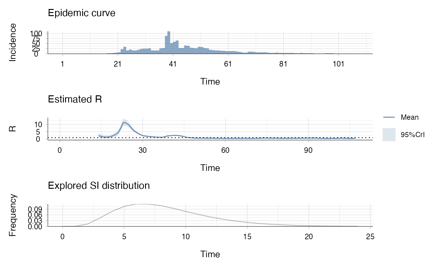
plot(res_weekly)
 ## Example using repeating vector of aggregation windows e.g. for consistent
## reporting 3 times a week
# Using the SARS data again
data("SARS2003")
# For this example we will pretend data is being reported three times a week,
# in 2-day, 2-day, 3-day aggregations
incid <- SARS2003$incidence
dt <- c(2L,2L,3L)
agg_incid <- aggregate_inc(incid, dt)
#> Incidence aggregated up to day 107 of 107
si_distr <- SARS2003$si_distr
# estimate Rt using the default parameters (method "non_parametric_si")
method <- "non_parametric_si"
config <- make_config(list(si_distr = si_distr))
res_agg <- estimate_R_agg(incid = agg_incid,
dt = c(2L,2L,3L), # aggregation windows of the data
dt_out = 7L, # desired sliding window length
iter = 10L,
config = config,
method = method,
grid = list(precision = 0.001, min = -1, max = 1))
#> Warning: You're estimating R too early in the epidemic to get the desired
#> posterior CV.
#> Estimated R for iteration: 1
#> Reconstructed incidence for iteration: 1
#> Warning: You're estimating R too early in the epidemic to get the desired
#> posterior CV.
#> Estimated R for iteration: 2
#> Reconstructed incidence for iteration: 2
#> Warning: You're estimating R too early in the epidemic to get the desired
#> posterior CV.
#> Estimated R for iteration: 3
#> Reconstructed incidence for iteration: 3
#> Warning: You're estimating R too early in the epidemic to get the desired
#> posterior CV.
#> Estimated R for iteration: 4
#> Reconstructed incidence for iteration: 4
#> Warning: You're estimating R too early in the epidemic to get the desired
#> posterior CV.
#> Estimated R for iteration: 5
#> Reconstructed incidence for iteration: 5
#> Warning: You're estimating R too early in the epidemic to get the desired
#> posterior CV.
#> Estimated R for iteration: 6
#> Reconstructed incidence for iteration: 6
#> Warning: You're estimating R too early in the epidemic to get the desired
#> posterior CV.
#> Estimated R for iteration: 7
#> Reconstructed incidence for iteration: 7
#> Warning: You're estimating R too early in the epidemic to get the desired
#> posterior CV.
#> Estimated R for iteration: 8
#> Reconstructed incidence for iteration: 8
#> Warning: You're estimating R too early in the epidemic to get the desired
#> posterior CV.
#> Estimated R for iteration: 9
#> Reconstructed incidence for iteration: 9
#> Warning: You're estimating R too early in the epidemic to get the desired
#> posterior CV.
#> Estimated R for iteration: 10
#> Reconstructed incidence for iteration: 10
#> Warning: You're estimating R too early in the epidemic to get the desired
#> posterior CV.
#> R estimation starts on day 8
# Plot the result
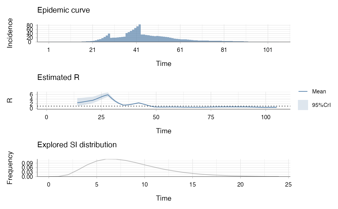
plot(res_agg)
## Example using repeating vector of aggregation windows e.g. for consistent
## reporting 3 times a week
# Using the SARS data again
data("SARS2003")
# For this example we will pretend data is being reported three times a week,
# in 2-day, 2-day, 3-day aggregations
incid <- SARS2003$incidence
dt <- c(2L,2L,3L)
agg_incid <- aggregate_inc(incid, dt)
#> Incidence aggregated up to day 107 of 107
si_distr <- SARS2003$si_distr
# estimate Rt using the default parameters (method "non_parametric_si")
method <- "non_parametric_si"
config <- make_config(list(si_distr = si_distr))
res_agg <- estimate_R_agg(incid = agg_incid,
dt = c(2L,2L,3L), # aggregation windows of the data
dt_out = 7L, # desired sliding window length
iter = 10L,
config = config,
method = method,
grid = list(precision = 0.001, min = -1, max = 1))
#> Warning: You're estimating R too early in the epidemic to get the desired
#> posterior CV.
#> Estimated R for iteration: 1
#> Reconstructed incidence for iteration: 1
#> Warning: You're estimating R too early in the epidemic to get the desired
#> posterior CV.
#> Estimated R for iteration: 2
#> Reconstructed incidence for iteration: 2
#> Warning: You're estimating R too early in the epidemic to get the desired
#> posterior CV.
#> Estimated R for iteration: 3
#> Reconstructed incidence for iteration: 3
#> Warning: You're estimating R too early in the epidemic to get the desired
#> posterior CV.
#> Estimated R for iteration: 4
#> Reconstructed incidence for iteration: 4
#> Warning: You're estimating R too early in the epidemic to get the desired
#> posterior CV.
#> Estimated R for iteration: 5
#> Reconstructed incidence for iteration: 5
#> Warning: You're estimating R too early in the epidemic to get the desired
#> posterior CV.
#> Estimated R for iteration: 6
#> Reconstructed incidence for iteration: 6
#> Warning: You're estimating R too early in the epidemic to get the desired
#> posterior CV.
#> Estimated R for iteration: 7
#> Reconstructed incidence for iteration: 7
#> Warning: You're estimating R too early in the epidemic to get the desired
#> posterior CV.
#> Estimated R for iteration: 8
#> Reconstructed incidence for iteration: 8
#> Warning: You're estimating R too early in the epidemic to get the desired
#> posterior CV.
#> Estimated R for iteration: 9
#> Reconstructed incidence for iteration: 9
#> Warning: You're estimating R too early in the epidemic to get the desired
#> posterior CV.
#> Estimated R for iteration: 10
#> Reconstructed incidence for iteration: 10
#> Warning: You're estimating R too early in the epidemic to get the desired
#> posterior CV.
#> R estimation starts on day 8
# Plot the result
plot(res_agg)
 ## Example using full vector of aggregation windows
dt <- rep(c(2L,2L,3L), length.out=length(agg_incid))
si_distr <- SARS2003$si_distr
# estimate Rt using the default parameters (method "non_parametric_si")
method <- "non_parametric_si"
config <- make_config(list(si_distr = si_distr))
res_agg <- estimate_R_agg(incid = agg_incid,
dt = dt, # aggregation windows of the data
dt_out = 7L, # desired sliding window length
iter = 10L,
config = config,
method = method,
grid = list(precision = 0.001, min = -1, max = 1))
#> Warning: You're estimating R too early in the epidemic to get the desired
#> posterior CV.
#> Estimated R for iteration: 1
#> Reconstructed incidence for iteration: 1
#> Warning: You're estimating R too early in the epidemic to get the desired
#> posterior CV.
#> Estimated R for iteration: 2
#> Reconstructed incidence for iteration: 2
#> Warning: You're estimating R too early in the epidemic to get the desired
#> posterior CV.
#> Estimated R for iteration: 3
#> Reconstructed incidence for iteration: 3
#> Warning: You're estimating R too early in the epidemic to get the desired
#> posterior CV.
#> Estimated R for iteration: 4
#> Reconstructed incidence for iteration: 4
#> Warning: You're estimating R too early in the epidemic to get the desired
#> posterior CV.
#> Estimated R for iteration: 5
#> Reconstructed incidence for iteration: 5
#> Warning: You're estimating R too early in the epidemic to get the desired
#> posterior CV.
#> Estimated R for iteration: 6
#> Reconstructed incidence for iteration: 6
#> Warning: You're estimating R too early in the epidemic to get the desired
#> posterior CV.
#> Estimated R for iteration: 7
#> Reconstructed incidence for iteration: 7
#> Warning: You're estimating R too early in the epidemic to get the desired
#> posterior CV.
#> Estimated R for iteration: 8
#> Reconstructed incidence for iteration: 8
#> Warning: You're estimating R too early in the epidemic to get the desired
#> posterior CV.
#> Estimated R for iteration: 9
#> Reconstructed incidence for iteration: 9
#> Warning: You're estimating R too early in the epidemic to get the desired
#> posterior CV.
#> Estimated R for iteration: 10
#> Reconstructed incidence for iteration: 10
#> Warning: You're estimating R too early in the epidemic to get the desired
#> posterior CV.
#> R estimation starts on day 8
# Plot the result
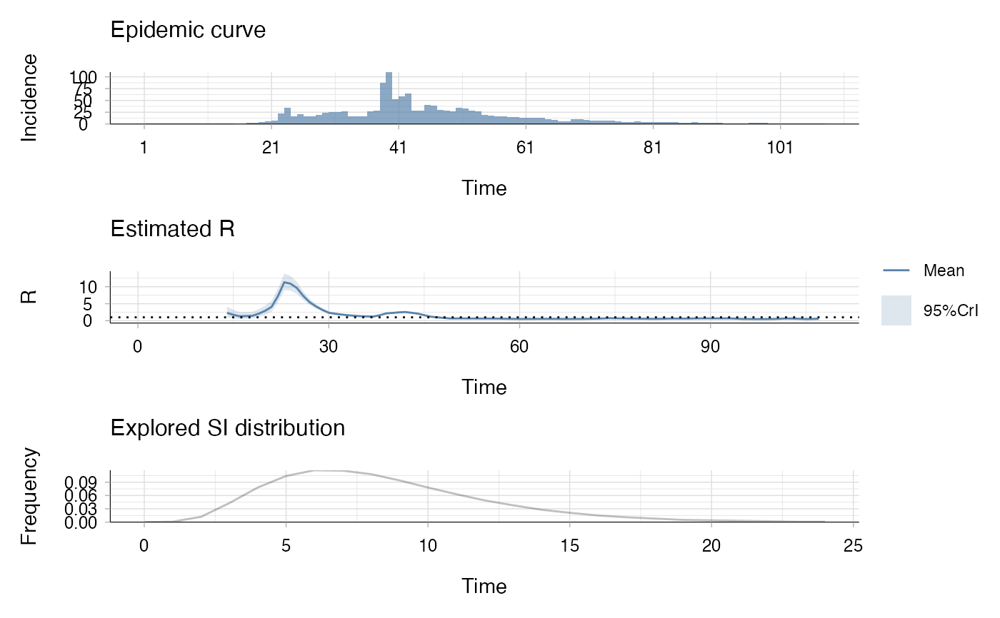
plot(res_agg)
## Example using full vector of aggregation windows
dt <- rep(c(2L,2L,3L), length.out=length(agg_incid))
si_distr <- SARS2003$si_distr
# estimate Rt using the default parameters (method "non_parametric_si")
method <- "non_parametric_si"
config <- make_config(list(si_distr = si_distr))
res_agg <- estimate_R_agg(incid = agg_incid,
dt = dt, # aggregation windows of the data
dt_out = 7L, # desired sliding window length
iter = 10L,
config = config,
method = method,
grid = list(precision = 0.001, min = -1, max = 1))
#> Warning: You're estimating R too early in the epidemic to get the desired
#> posterior CV.
#> Estimated R for iteration: 1
#> Reconstructed incidence for iteration: 1
#> Warning: You're estimating R too early in the epidemic to get the desired
#> posterior CV.
#> Estimated R for iteration: 2
#> Reconstructed incidence for iteration: 2
#> Warning: You're estimating R too early in the epidemic to get the desired
#> posterior CV.
#> Estimated R for iteration: 3
#> Reconstructed incidence for iteration: 3
#> Warning: You're estimating R too early in the epidemic to get the desired
#> posterior CV.
#> Estimated R for iteration: 4
#> Reconstructed incidence for iteration: 4
#> Warning: You're estimating R too early in the epidemic to get the desired
#> posterior CV.
#> Estimated R for iteration: 5
#> Reconstructed incidence for iteration: 5
#> Warning: You're estimating R too early in the epidemic to get the desired
#> posterior CV.
#> Estimated R for iteration: 6
#> Reconstructed incidence for iteration: 6
#> Warning: You're estimating R too early in the epidemic to get the desired
#> posterior CV.
#> Estimated R for iteration: 7
#> Reconstructed incidence for iteration: 7
#> Warning: You're estimating R too early in the epidemic to get the desired
#> posterior CV.
#> Estimated R for iteration: 8
#> Reconstructed incidence for iteration: 8
#> Warning: You're estimating R too early in the epidemic to get the desired
#> posterior CV.
#> Estimated R for iteration: 9
#> Reconstructed incidence for iteration: 9
#> Warning: You're estimating R too early in the epidemic to get the desired
#> posterior CV.
#> Estimated R for iteration: 10
#> Reconstructed incidence for iteration: 10
#> Warning: You're estimating R too early in the epidemic to get the desired
#> posterior CV.
#> R estimation starts on day 8
# Plot the result
plot(res_agg)