Fitting rainfall profiles

library(umbrella)

Below is an example workflow for using the umbrella package to fit rainfall profiles for use in malariasimulation. Fitting a Fourier series provides a smooth representation of seasonal rainfall patterns that can be supplied directly to the malariasimulation package.

First you’ll need to download the rasters and extract the raw data. There are some helper functions to download global daily rainfall rasters in the package. You can use the get_urls() function to create the URLs to get daily rainfall rasters for a given year. After that the download_raster() can be used to download the rasters to your device. Beware that the set of unzipped rasters for a whole year will take up quite a bit of memory (each raster is about 2.2 MB).

Once you have your set of rasters you can load them and extract the data. For this I recommend getting a sf shape file with the boundaries of the area you would like to extract the data for. The R package terra is a great way to extract the data, something like: Many openly available administrative boundary shapefiles can be obtained from resources such as GADM or Natural Earth.

my_raster_files <- c("rainfall1.tif", "rainfall2.tif")
my_raster <- terra::rast(my_raster_files)
my_sf <- load("my_sf.rds")
extract_data <- terra::extract(my_raster, my_sf, fun = mean)

Once you’ve extracted and tidied the output, you might have something like:

head(rainfall)
#>   day rainfall
#> 1   1     0.00
#> 2   2     0.00
#> 3   3     0.00
#> 4   4     0.28
#> 5   5     0.17
#> 6   6     0.03

The built-in rainfall data set contains 365 rows with two columns: day, giving the day of the year, and rainfall, giving the observed rainfall in millimetres at a single location. We’ll use it here to demonstrate fitting seasonal profiles.

Let’s fit a simple seasonal profile to this dataset, and a profile with an imposed minimum rainfall floor.

fit1 <- fit_fourier(rainfall = rainfall$rainfall, t = rainfall$day, floor = 0)
predict_1 <- fourier_predict(coef = fit1$coefficients, t = 1:365, floor = 0)

fit2 <- fit_fourier(rainfall = rainfall$rainfall, t = rainfall$day, floor = 1)
predict_2 <- fourier_predict(coef = fit2$coefficients, t = 1:365, floor = 1)

plot(rainfall, xlab = "Day", ylab = "Rainfall", pch = 19)
lines(predict_1, col = "deeppink", lwd = 2)
lines(predict_2, col = "dodgerblue", lwd = 2, lty = 2)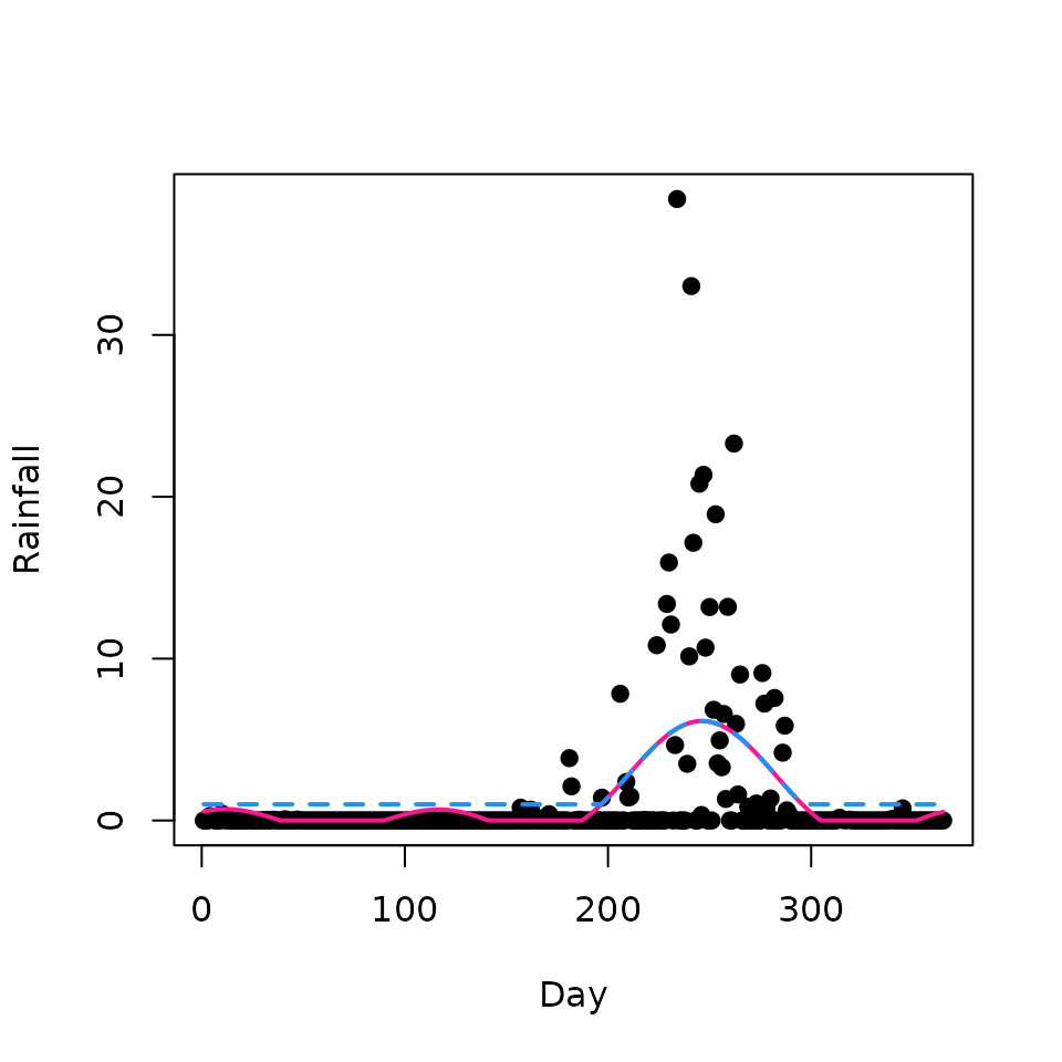

The pink line shows the profile fitted without imposing a minimum rainfall value. The dashed blue line applies a floor of 1 mm and therefore never drops below that value.