Analysing malariasimulation output with postie

Postie provides tools to post-process output from malariasimulation. This vignette runs a short example simulation and explores how to summarise the resulting prevalence and incidence estimates.

Running a basic simulation

# install.packages("malariasimulation")
library(malariasimulation)
library(postie)
library(dplyr)
#> 
#> Attaching package: 'dplyr'
#> The following objects are masked from 'package:stats':
#> 
#>     filter, lag
#> The following objects are masked from 'package:base':
#> 
#>     intersect, setdiff, setequal, union
library(ggplot2)

# set up parameters
year <- 365
p <- get_parameters() |>
  set_drugs(list(AL_params)) |>
  set_clinical_treatment(1, 0.5, 0.5) |>
  set_epi_outputs(
    age_group = c(0, 5, 15, 200) * year,
    prevalence = c(2, 10) * year,
    clinical_incidence = c(0, 5, 15, 200) * year,
    severe_incidence = c(0, 5, 15, 200) * year
  )

# run for two years
sim <- run_simulation(2 * year, p)

The object sim is a data frame containing the time series of all requested outputs. Postie converts these counts into rates that are easier to interpret.

Rates and prevalence

rates <- get_rates(sim)
#> Warning in get_rates(sim): required column `ft_sev` (probability
#> hospitalisation | severe case) not found, assuming ft_sev = 0.8
#> Warning: required column `ft_sev` (probability hospitalisation | severe case) not found, assuming ft_sev = 0.8
head(rates)
#> # A tibble: 6 × 18
#>    year month  week   day  time age_lower age_upper clinical severe_hospital
#>   <dbl> <int> <dbl> <dbl> <dbl>     <dbl>     <dbl>    <dbl>           <dbl>
#> 1  2000     1     1     1 2000          0      5.00        0               0
#> 2  2000     1     1     1 2000          5     15.0         0               0
#> 3  2000     1     1     1 2000         15    200.          0               0
#> 4  2000     1     1     2 2000.         0      5.00        0               0
#> 5  2000     1     1     2 2000.         5     15.0         0               0
#> 6  2000     1     1     2 2000.        15    200.          0               0
#> # ℹ 9 more variables: severe_community <dbl>, severe <dbl>,
#> #   mortality_hospital <dbl>, mortality_community <dbl>, mortality <dbl>,
#> #   yld <dbl>, yll <dbl>, dalys <dbl>, person_days <dbl>

sim <- dplyr::mutate(sim, ft_sev = 0.5)
rates <- get_rates(sim)

prev <- get_prevalence(sim)
head(prev)
#>   year month week day     time lm_prevalence_2_10
#> 1 2000     1    1   1 2000.000          0.5185185
#> 2 2000     1    1   2 2000.003          0.5185185
#> 3 2000     1    1   3 2000.005          0.5185185
#> 4 2000     1    1   4 2000.008          0.5185185
#> 5 2000     1    1   5 2000.011          0.5185185
#> 6 2000     1    1   6 2000.014          0.5185185

Handling ft_sev

The column ft_sev contains the probability that a severe case leads to hospital admission. When it is missing get_rates() assumes a value of 0.8 and prints a warning. By supplying your own column before calling the function you can control this assumption and remove the warning.

For the full methodology behind how postie adjusts severe incidence and derives mortality from ft_sev (and the related treatment_scaler, hosp_sev_cfr and community_sev_cfr arguments), see the vignette("severe-mortality").

The rates are per person per day. Multiplying by 365 converts them to the more familiar per person per year units.

prev |>
  ggplot(aes(time, lm_prevalence_2_10)) +
  theme_bw() +
  geom_line() +
  labs(y = expression(PfPr[2-10]))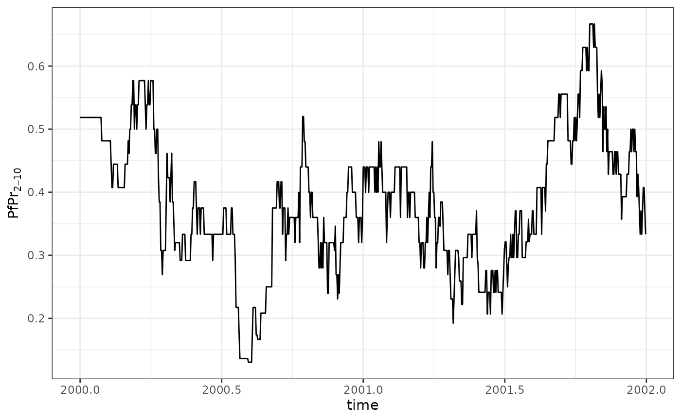

Units and time aggregation

Rates returned by get_rates() are expressed per person per day. The unit is separate from the time interval over which values are aggregated. You can therefore average rates by month or year while still reporting them as cases per person per year by multiplying by 365.

Aggregating over time and age

The flexibility of postie means you can aggregate outputs in many ways. For example, to obtain annual clinical incidence and mortality by the three age groups:

summary <- rates |>
  mutate(
    age_group = case_when(
      age_upper <= 5 ~ "U5",
      age_upper <= 15 ~ "5-15",
      TRUE ~ "15+"
    )
  ) |>
  summarise(
    clinical = weighted.mean(clinical, person_days) * 365,
    mortality = weighted.mean(mortality, person_days) * 365,
    person_days = sum(person_days),
    time = mean(time),
    .by = c(year, age_group)
  )
summary
#> # A tibble: 6 × 6
#>    year age_group clinical mortality person_days  time
#>   <dbl> <chr>        <dbl>     <dbl>       <dbl> <dbl>
#> 1  2000 U5            1.32   0.0311         8047 2000.
#> 2  2000 5-15          5.19   0.0293        12809 2000.
#> 3  2000 15+           3.50   0.0320        15644 2000.
#> 4  2001 U5            1.30   0.0159         7884 2001.
#> 5  2001 5-15          3.02   0.0197        12674 2001.
#> 6  2001 15+           2.82   0.00785       15942 2001.

Aggregating by both year and month can reveal seasonal patterns. The following code collapses the daily values to monthly rates and plots the clinical incidence over time.

monthly <- rates |>
  summarise(
    clinical = weighted.mean(clinical, person_days) * 365,
    time = mean(time),
    .by = c(year, month)
  )

monthly |>
  ggplot(aes(time, clinical)) +
  theme_bw() +
  geom_line() +
  labs(y = "clinical per person per year")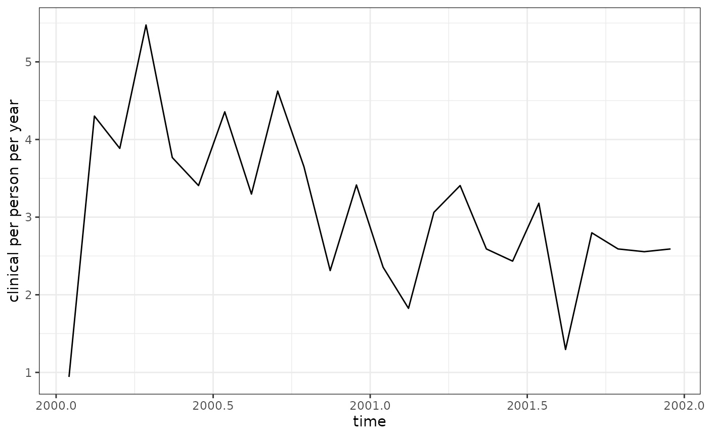

Postie therefore provides a straightforward pipeline from raw model output to tidy, aggregated indicators ready for further analysis or visualisation.