Converting between bed net metrics • netz

There are many different metrics associated with measuring bed net “coverage”.

These metrics are summarised in an excellent paper by Amelia Bertozzi-Villa and collegues:

Bertozzi-Villa, Amelia, et al. Nature communications 12.1 (2021): 1-12, please check it out and make sure to cite appropriately if you use this package.

We define them here as:

Usage: The proportion of the population with a net who slept under it.
Access: The proportion of the population who live in a household where they could sleep under a bed net.
Crop: The number of nets in the population. Always expressed as nets per capita.
Distribution: The number of nets distributed. Always expressed as nets per capita.

Being able to convert between these metrics is useful for a number of reasons:

If you have data for one, but need information for another
If a specific metric is requested as an output
If you are trying to align with estimates that use the same underlying model
If your work requires costing of bed net distributions

Conversion steps

The conversion from net usage to annual nets distributed per capita occurs in the following steps:

Usage ⬅️➡️ Access

Convert between net usage and net access using either an estimated country-specific
or a user-specified use rate. By definition, net use rate = net usage/net access.

Access ⬅️➡️ Crop

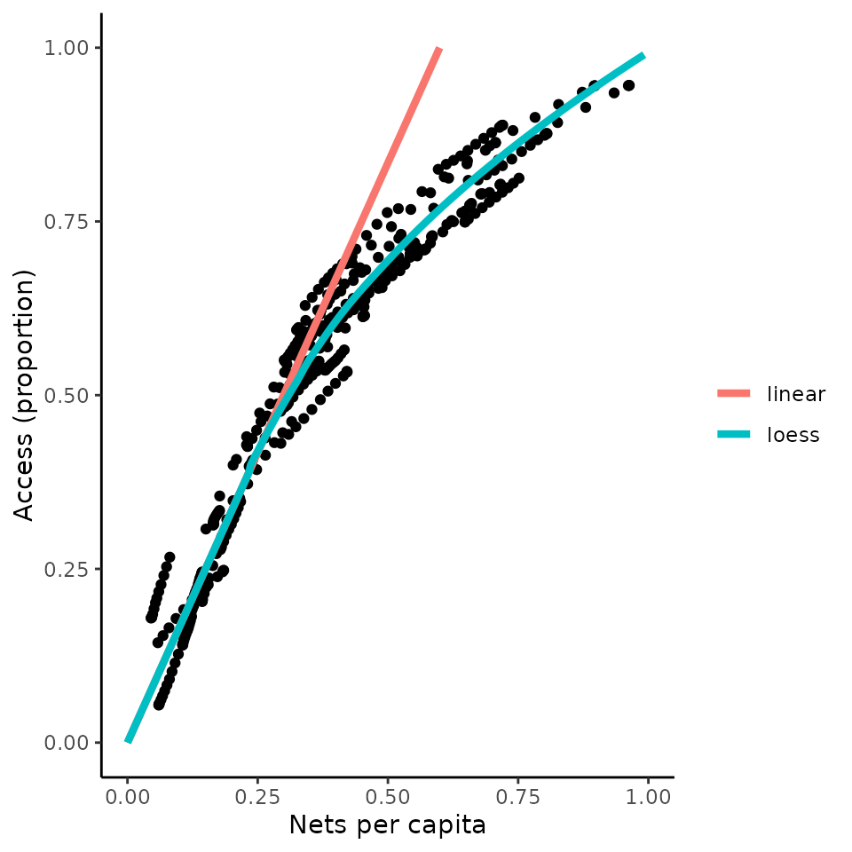
Convert between net access and net crop using either a linear-relationship based on the number of people that can use one net, or a Loess curve fitted to the observed relationship between these two metrics across sub-Saharan Africa.

Crop ⬅️➡️ Distribution

Convert between net crop and net distributions accounting for net distribution timing and net loss over time.

Conversion example

We can demonstrate an example of a simple conversion of this kind

# Create some example data for net usage in Nigeria over 4 years
iso3c <- "NGA"
years <- 2000:2003
usage <- c(0.1, 0.2, 0.6, 0.5)
output <- 
  data.frame(
    year = years,
    iso3c = iso3c,
    usage = usage
  )

# Access the estimates of usage rate and net-retention half life for Nigeria
usage_rate <- get_usage_rate(iso3c)
half_life <- get_halflife(iso3c)

# Use the nets functionality to convert usage ➡️ acesss ➡️ crop ➡️ distribution
output$access <- usage_to_access(
  usage = output$usage, 
  use_rate = usage_rate
  )
output$crop <- access_to_crop(
  access = output$access,
  type = "loess"
  )
output$distribution <- crop_to_distribution(
  crop = output$crop,
  crop_timesteps = (output$year + 0.5) * 365,
  distribution_timesteps = (output$year) * 365,
  half_life = half_life
)

output
#>   year iso3c usage    access       crop distribution
#> 1 2000   NGA   0.1 0.1136881 0.06813548   0.07048166
#> 2 2001   NGA   0.2 0.2273763 0.13627097   0.08748988
#> 3 2002   NGA   0.6 0.6821289 0.48564537   0.40593797
#> 4 2003   NGA   0.5 0.5684407 0.36434064   0.01972797

And, if we want we can make the same conversions in the opposite direction

output <- output[, c("year", "iso3c", "distribution")]

# Use the nets functionality to convert distribution ➡️ crop ➡️ access ➡️ usage
output$crop <- distribution_to_crop(
  distribution = output$distribution,
  distribution_timesteps = (output$year) * 365,
  crop_timesteps = (output$year + 0.5) * 365,
  half_life = half_life
)
output$access <- crop_to_access(
  crop = output$crop,
  type = "loess"
)
output$usage <- access_to_usage(
  access = output$access,
  use_rate = usage_rate
)

# We retrieve our original input usage:
round(output$usage, 2)
#> [1] 0.1 0.2 0.6 0.5

The relationship between access and crop

The relationship between access and crop is derived from monthly data for the latest available year (2020) across African countries, and plotted below (corresponding to Figure 4 in the paper by Bertozzi-Villa et al). There are two options in the access_to_crop() function one “loess” a loess smooth of the data extrapolated to allow prediction for access values outside of the observed range and a second, “linear”, which assumed a fixed number of people can use each net. The linear model is very simple and does not fit the observed data well, so use with caution, although it is often the way bed nets are costed.

library(ggplot2)
access <- seq(0, 1, 0.01)
crop_loess <- access_to_crop(access, type = "loess")
crop_linear <- access_to_crop(access, type = "linear")
model_data <- data.frame(access = rep(access, 2),
                         model = rep(c("loess", "linear"), each = length(crop_loess)),
                         crop = c(crop_loess, crop_linear))

# Plot curve
ggplot() +
  geom_point(
    data = crop_data,
    aes(x = percapita_nets_mean, y = access_mean),
    col = "black"
    ) +
  geom_line(
    data = model_data,
    aes(x = crop, y = access, colour = model),
    size = 1.5
    ) +
  xlim(0, 1) +
  ylim(0, 1) +
  labs(x = "Nets per capita", y = "Access (proportion)", colour = "") +
  theme_classic()

Assumptions about the net loss function

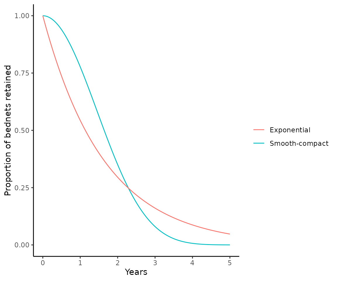
The default option in these metric conversions assumes that nets are lost according to a smooth-compact function (net_loss_function = net_loss_map). This in line with the paper by Bertozzi-Villa et al.

An alternative option is to assume exponential net loss (net_loss_function = net_loss_exp), which corresponds to the assumption in malariasimulation.

The proportion of nets retained over time are visualised for both options below, for a 3 year distribution cycle and a net half life of 1.64 years.

t <- seq(0, 5 * 365, 1)

# Calculate proportion of nets retained assuming smooth-compact net loss
nets_retained_map <- net_loss_map(
  t = t,
  k = 20,
  half_life = 1.64 * 365
)
# k is a fixed rate parameter based on which net half lives were estimated in the paper

# Calculate proportion of nets retained assuming exponential net loss
nets_retained_exp <- net_loss_exp(
  t = t,
  mean_retention = 1.64 * 365
)

# Plot curve
ggplot() +
  geom_line(aes(
    x = t / 365, y = nets_retained_map,
    colour = "Smooth-compact"
  )) +
  geom_line(aes(
    x = t / 365, y = nets_retained_exp,
    colour = "Exponential"
  )) +
  ylim(0, 1) +
  labs(x = "Years", y = "Proportion of bednets retained", colour = "") +
  theme_classic()