Getting started

Running the model

First we will run the model without vaccination.

Start by reading in your table of parameters:

 library("gonovax")
#> 
#> Attaching package: 'gonovax'
#> The following object is masked from 'package:stats':
#> 
#>     aggregate
#> The following object is masked from 'package:base':
#> 
#>     transform
 parameter_table <- read.csv("../inst/extdata/gono_params_t.csv")
 head(parameter_table)
#>        beta     eta_l     eta_h   epsilon        mu       nu        psi
#> 1 0.5548627 0.3443120 0.7972842 0.6424030 209.93828 4.959542 0.09410734
#> 2 0.3170303 0.3801225 0.5502756 0.5980645 367.67133 2.186269 0.15101774
#> 3 0.3539354 0.4109142 0.5373065 0.8849614 326.20064 2.352640 0.12483779
#> 4 0.3103453 0.3766348 0.7828353 0.4517068 187.20356 1.923302 0.19032818
#> 5 0.4528126 0.3873987 0.7570947 0.7225662  96.52862 3.765360 0.12384225
#> 6 0.6251540 0.3599922 0.5629054 0.6053695 255.82950 4.711401 0.08233706
#>        rho     sigma   prev_Ash    prev_Asl
#> 1 51.29849  46.42424 0.07490694 0.001812143
#> 2 62.06935  80.99252 0.06012777 0.009626622
#> 3 56.91546 155.36248 0.06817730 0.008933017
#> 4 46.38395  69.83441 0.05306220 0.007125388
#> 5 73.68399 132.37154 0.03265509 0.008589632
#> 6 53.32993  74.55650 0.07191239 0.002668673

We need to transform the table of parameters to the format the model requires using the transform_fixed function. First we only use 100 parameter sets:

n_par <- 100

# transform the parameter table
gono_params <- lapply(seq_len(n_par),
                      function(i) transform_fixed(parameter_table[i, ]))

We then run the model to equilibrium without vaccination, and save the final states for each parameter set so we can restart with vaccination:

# define the times of the output (in years)
tt <- c(0, 50)

# run the model
y0 <- run_onevax_xvwv(tt, gono_params)

# get final (equilibrium) model state for restart
init_params <- lapply(y0, restart_params)

We now run the model with vaccination.

The efficacy inputs (vea, vei, ved, ves) can be of length 1 or n_par

The strategy can be one of; VoD: vaccination on diagnosis VoA: vaccination on attendance * VoD(L)+VoA(H): targeted vaccination (i.e. all diagnosed plus group H on screening)

The proportion of those eligible that choose to be vaccinated, uptake is a scalar from 0 - 1:

# generate vaccine effects parameters
ve <- data.frame(vea = 0.1, # efficacy against acquisition
                 vei = 0.2, # efficacy against infectiousness
                 ved = 0.3, # efficacy against duration of infection
                 ves = 0.4) # efficacy against symptoms

tt <- seq(0, 10)
y <- run_onevax_xvwv(tt,
                     gono_params = gono_params,
                     init_params = init_params, 
                     vea = ve$vea, ved = ve$ved, ves = ve$ves,
                     uptake = 1, strategy = "VoA")

y is now a list of model runs of length n_par, each entry contains a list of model outputs. Each of these list entries y[[i]] is a list of model output arrays with dimensions: time, group (L, H), and vaccine status (X, V, W) where applicable

names(y[[1]])
#>  [1] "t"              "U"              "I"              "A"             
#>  [5] "S"              "T"              "cum_incid"      "cum_diag_a"    
#>  [9] "cum_diag_s"     "cum_treated"    "cum_screened"   "cum_vaccinated"
#> [13] "tot_treated"    "tot_attended"   "beta"           "eta"           
#> [17] "lambda"         "N"
dim(y[[1]]$cum_incid)
#> [1] 11  2  3
dimnames(y[[1]]$cum_incid)
#> [[1]]
#> NULL
#> 
#> [[2]]
#> [1] "L" "H"
#> 
#> [[3]]
#> [1] "X" "V" "W"

# cumulative incidence in unvaccinated group L over time
y[[1]]$cum_incid[, "L", "X"]
#>  [1]     0.00 12019.16 17752.48 20517.99 21988.09 22851.44 23405.84 23790.58
#>  [9] 24076.17 24301.00 24487.20

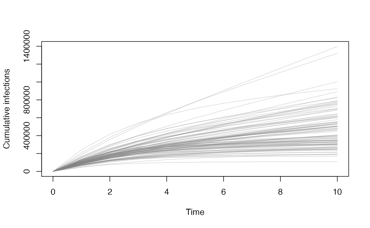
This will aggregate over group (L, H) and strata (X, V, W) to give the total cumulative infections for each parameter set (rows) over time (columns).

total_infected <- aggregate(y, what = "cum_incid")
col <- rgb(0.5, 0.5, 0.5, 0.3)
matplot(tt, t(total_infected), lty = 1, type = "l", col = col,
        xlab = "Time", ylab = "Cumulative infections")

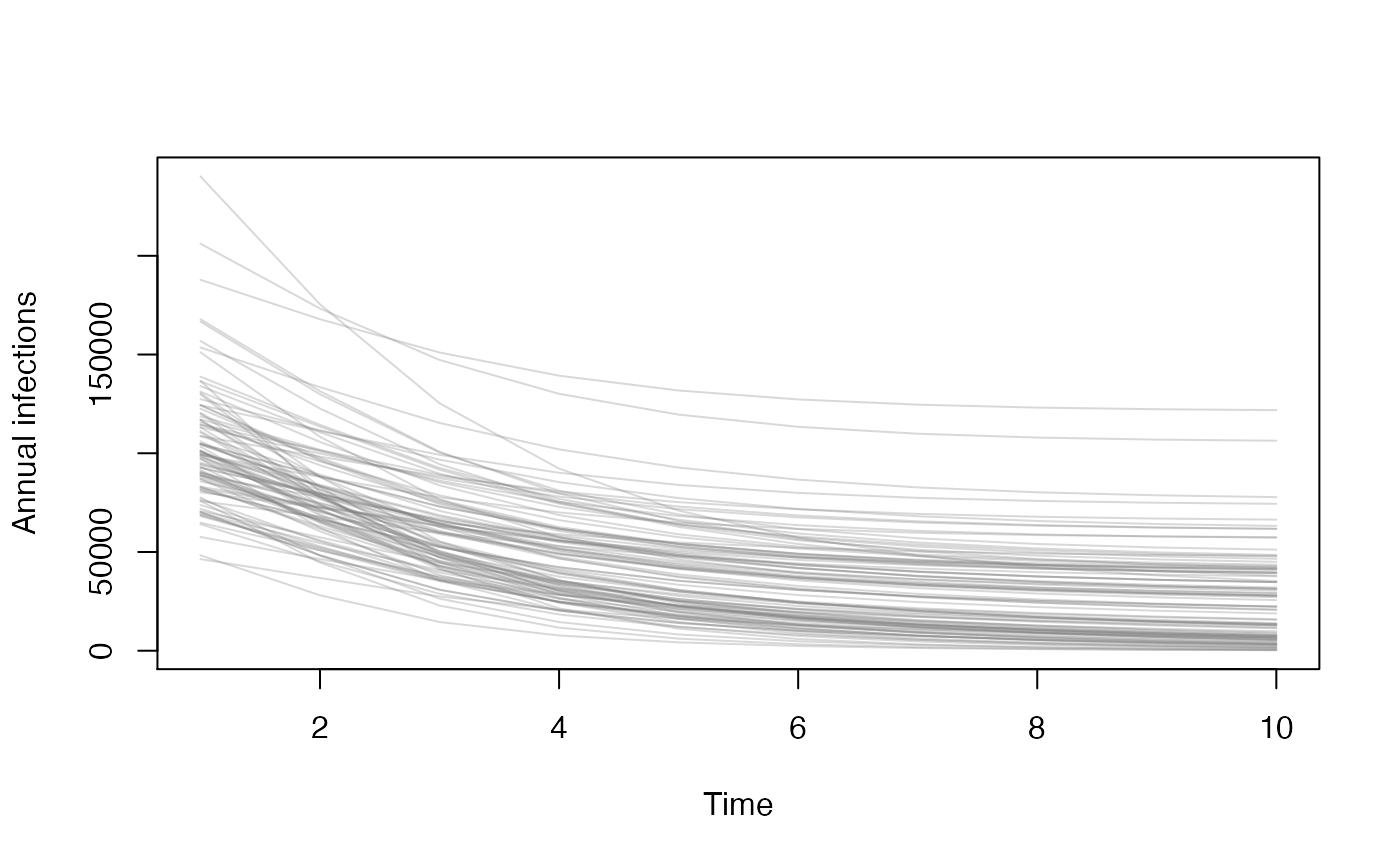
This will aggregate over group (L, H) and strata (X, V, W) to give the yearly infections for each parameter set (rows) over time (columns)

annual_infected <- aggregate(y, what = "cum_incid", as_incid = TRUE)
matplot(tt[-1], t(annual_infected), lty = 1, type = "l", col = col,
        xlab = "Time", ylab = "Annual infections")

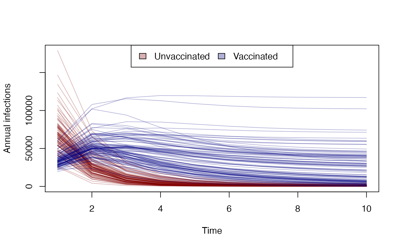
You can look at individual vaccine strata:

annual_infected_X <- aggregate(y, what = "cum_incid", as_incid = TRUE,
                             stratum = "X")
annual_infected_V <- aggregate(y, what = "cum_incid", as_incid = TRUE,
                             stratum = "V")
col1 <- rgb(0.5, 0, 0, 0.3)
col2 <- rgb(0, 0, 0.5, 0.3)
matplot(tt[-1], t(annual_infected_X), lty = 1, type = "l", col = col1,
        xlab = "Time", ylab = "Annual infections")
matlines(tt[-1], t(annual_infected_V), lty = 1, col = col2)
legend("top", fill = c(col1, col2), legend = c("Unvaccinated", "Vaccinated"),
       ncol = 2)

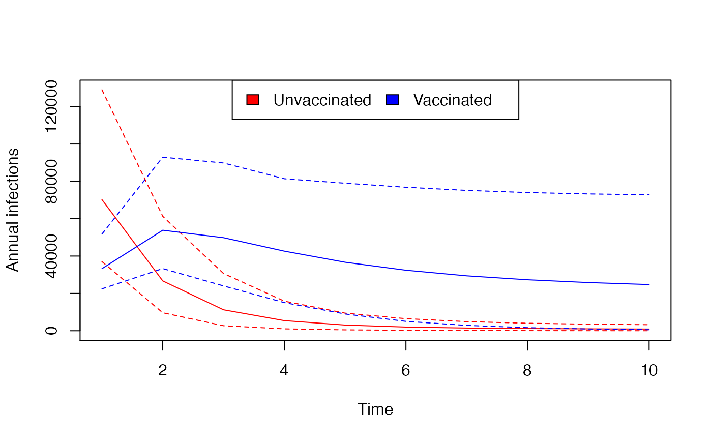
You can look apply functions over the parameter sets to get summary statistics

mean_ci <- function(x) c(mean = mean(x), quantile(x, c(0.025, 0.975)))
summary_annual_infected_X <- aggregate(y, what = "cum_incid", as_incid = TRUE,
                             stratum = "X", f = mean_ci)
summary_annual_infected_V <- aggregate(y, what = "cum_incid", as_incid = TRUE,
                             stratum = "V", f = mean_ci)
col1 <- "red"
col2 <- "blue"
matplot(tt[-1], t(summary_annual_infected_X), lty = c(1, 2, 2), type = "l", col = col1,
        xlab = "Time", ylab = "Annual infections")
matlines(tt[-1], t(summary_annual_infected_V), lty = c(1, 2, 2), col = col2)
legend("top", fill = c(col1, col2), legend = c("Unvaccinated", "Vaccinated"),
       ncol = 2)

Lilith Whittles

2021-06-16

Running the model