PlasmoSim returns two types of output:
- Population-level data giving basic epidemiological measures (e.g. prevalence) on each day of simulation
- Individual-level data, including parasite genotypes found in the host at specific sampling points
This tutorial gives example of both outputs, and shows basic visualisation and interpretation functions.
Load necessary packages:
Daily trends
First, we need to define our desired sampling strategy using a data.frame. This specifies the demes (partially isolated sub-populations) that we will sample from, at what time points, and how many hosts will be drawn at random from the population:
# define individual-level sampling via a data.frame
sample_df <- data.frame(deme = 1,
                        time = 365,
                        n = 100)
Now we run the main simulation function:
# run simulation
sim1 <- sim_falciparum(H = 1000,                     # human population size
                       M = 5000,                     # adult female mosquito population size
                       seed_infections = 100,        # number of infected hosts at time 0
                       L = 24,                       # number of loci
                       sample_dataframe = sample_df  # sampling data.frame
                       )
#> Running simulation
#>
#> simulation completed in 0.044977 seconds
#> processing output
Daily output is stored in long format, which makes it easy to produce plots:
# basic plot of prevalence in "I" state (infected)
sim1$daily_values |>
  ggplot() + theme_bw() +
  geom_line(aes(x = time, y = 100 * I / 1000)) +
  ylab("Prevalence (%)")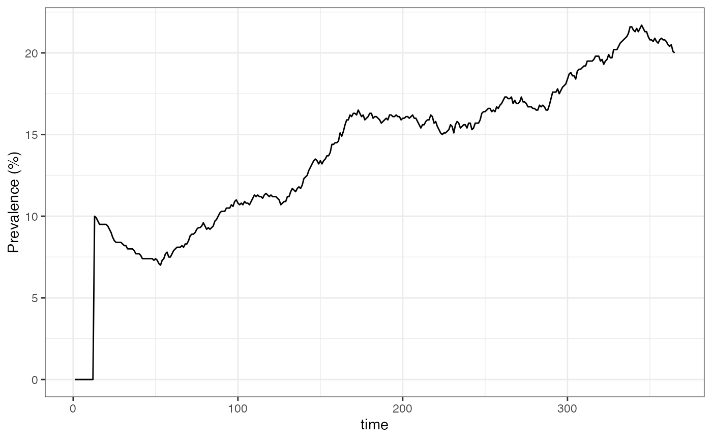
We can see that prevalence jumped to 10% (100 infected hosts in the population of 1000) on day 13. This is because we set the simulation going with 100 seed infections, which here means new liver-stage infections. The default time from liver-stage to blood-stage (the intrinsic incubation period) is set to by default, hence these all emerging together on day 13. After this point we can see dynamic and stochastic changes in the number infected.
Individual-level output
Individual-level output is also returned in long format. We will use
the kable package to make this slightly easier to read:
# take a peek at basic individual-level output, without the haplotypes column
sim1$indlevel |>
  kable() |>
  kable_styling(bootstrap_options = c("striped", "hover", "condensed")) |>
scroll_box(width = "1000px", height = "400px")| time | deme | sample_ID | positive | haplotypes | haplo_ID |
|---|---|---|---|---|---|
| 365 | 1 | 4 | TRUE | 53, 49, 53, 49, 53, 49, 53, 49, 53, 49, 53, 49, 53, 49, 53, 49, 53, 49, 53, 49, 53, 49, 53, 49, 53, 49, 53, 49, 53, 49, 53, 49, 53, 49, 53, 49, 53, 49, 53, 49, 53, 49, 53, 49, 53, 49, 53, 49 | 0d05caa56fd36e9a1b89ec813cef6de7, aebf4c862e33f32175d67ea1da874083 |
| 365 | 1 | 11 | FALSE | NULL | NULL |
| 365 | 1 | 20 | FALSE | NULL | NULL |
| 365 | 1 | 24 | TRUE | 95, 20, 95, 20, 95, 20, 95, 20, 95, 20, 95, 20, 95, 20, 95, 20, 95, 20, 95, 20, 95, 20, 95, 20, 95, 20, 95, 20, 95, 20, 95, 20, 95, 20, 95, 20, 95, 20, 95, 20, 95, 20, 95, 20, 95, 20, 95, 20 | 9d388933684a98fd4aadb81853b7f428, e50f6a71c2afb9ed59b693190ad61627 |
| 365 | 1 | 27 | FALSE | NULL | NULL |
| 365 | 1 | 30 | FALSE | NULL | NULL |
| 365 | 1 | 31 | FALSE | NULL | NULL |
| 365 | 1 | 42 | TRUE | 42, 80, 42, 80, 42, 80, 42, 80, 42, 80, 42, 80, 42, 80, 42, 80, 42, 80, 42, 80, 42, 80, 42, 80, 42, 80, 42, 80, 42, 80, 42, 80, 42, 80, 42, 80, 42, 80, 42, 80, 42, 80, 42, 80, 42, 80, 42, 80 | e582bccedae1a8c866136c0c59119502, 31e13e2261febeadc3f96f949f2e8c64 |
| 365 | 1 | 44 | TRUE | 89, 89, 89, 89, 89, 89, 89, 89, 89, 89, 89, 89, 89, 89, 89, 89, 89, 89, 89, 89, 89, 89, 89, 89 | 4c364f6f36b13c5e685e9a946b2c38c1 |
| 365 | 1 | 45 | FALSE | NULL | NULL |
| 365 | 1 | 47 | FALSE | NULL | NULL |
| 365 | 1 | 50 | FALSE | NULL | NULL |
| 365 | 1 | 54 | FALSE | NULL | NULL |
| 365 | 1 | 60 | FALSE | NULL | NULL |
| 365 | 1 | 66 | FALSE | NULL | NULL |
| 365 | 1 | 68 | TRUE | 31, 31, 31, 31, 31, 31, 31, 31, 31, 31, 31, 31, 31, 31, 31, 31, 31, 31, 31, 31, 31, 31, 31, 31 | 47287a0c2513c31eb7c23142fcd993ad |
| 365 | 1 | 81 | FALSE | NULL | NULL |
| 365 | 1 | 86 | TRUE | 73, 73, 73, 73, 73, 73, 73, 73, 73, 73, 73, 73, 73, 73, 73, 73, 73, 73, 73, 73, 73, 73, 73, 73 | d970e356b0df023a5a26c8bdc1c7e017 |
| 365 | 1 | 87 | FALSE | NULL | NULL |
| 365 | 1 | 93 | FALSE | NULL | NULL |
| 365 | 1 | 103 | FALSE | NULL | NULL |
| 365 | 1 | 109 | FALSE | NULL | NULL |
| 365 | 1 | 110 | FALSE | NULL | NULL |
| 365 | 1 | 128 | FALSE | NULL | NULL |
| 365 | 1 | 147 | FALSE | NULL | NULL |
| 365 | 1 | 154 | FALSE | NULL | NULL |
| 365 | 1 | 168 | FALSE | NULL | NULL |
| 365 | 1 | 176 | FALSE | NULL | NULL |
| 365 | 1 | 177 | FALSE | NULL | NULL |
| 365 | 1 | 179 | FALSE | NULL | NULL |
| 365 | 1 | 181 | FALSE | NULL | NULL |
| 365 | 1 | 202 | FALSE | NULL | NULL |
| 365 | 1 | 203 | FALSE | NULL | NULL |
| 365 | 1 | 217 | FALSE | NULL | NULL |
| 365 | 1 | 220 | FALSE | NULL | NULL |
| 365 | 1 | 226 | FALSE | NULL | NULL |
| 365 | 1 | 258 | FALSE | NULL | NULL |
| 365 | 1 | 271 | TRUE | 65, 65, 65, 65, 65, 65, 65, 65, 65, 65, 65, 65, 65, 65, 65, 65, 65, 65, 65, 65, 65, 65, 65, 65 | 94a00c7081a586f1d9e7d2cadd066fb0 |
| 365 | 1 | 279 | FALSE | NULL | NULL |
| 365 | 1 | 282 | FALSE | NULL | NULL |
| 365 | 1 | 288 | FALSE | NULL | NULL |
| 365 | 1 | 311 | FALSE | NULL | NULL |
| 365 | 1 | 314 | FALSE | NULL | NULL |
| 365 | 1 | 318 | FALSE | NULL | NULL |
| 365 | 1 | 321 | TRUE | 64, 64, 64, 64, 64, 64, 64, 64, 64, 64, 64, 64, 64, 64, 64, 64, 64, 64, 64, 64, 64, 64, 64, 64 | 14e7f028287c07ea9e875126193d6aca |
| 365 | 1 | 333 | FALSE | NULL | NULL |
| 365 | 1 | 338 | FALSE | NULL | NULL |
| 365 | 1 | 356 | FALSE | NULL | NULL |
| 365 | 1 | 375 | FALSE | NULL | NULL |
| 365 | 1 | 384 | FALSE | NULL | NULL |
| 365 | 1 | 411 | FALSE | NULL | NULL |
| 365 | 1 | 415 | TRUE | 14, 65, 14, 65, 14, 65, 14, 65, 14, 65, 14, 65, 14, 65, 14, 65, 14, 65, 14, 65, 14, 65, 14, 65, 14, 65, 14, 65, 14, 65, 14, 65, 14, 65, 14, 65, 14, 65, 14, 65, 14, 65, 14, 65, 14, 65, 14, 65 | 5a04f475aaafb7d8d57fb74d15afdf98, 94a00c7081a586f1d9e7d2cadd066fb0 |
| 365 | 1 | 441 | TRUE | 73, 21, 73, 21, 73, 21, 73, 21, 73, 21, 73, 21, 73, 21, 73, 21, 73, 21, 73, 21, 73, 21, 73, 21, 73, 21, 73, 21, 73, 21, 73, 21, 73, 21, 73, 21, 73, 21, 73, 21, 73, 21, 73, 21, 73, 21, 73, 21 | d970e356b0df023a5a26c8bdc1c7e017, 5eba0a09b0d61a2da0d5bd4fffc6516f |
| 365 | 1 | 448 | FALSE | NULL | NULL |
| 365 | 1 | 460 | FALSE | NULL | NULL |
| 365 | 1 | 474 | FALSE | NULL | NULL |
| 365 | 1 | 485 | TRUE | 62, 62, 62, 62, 62, 62, 62, 62, 62, 62, 62, 62, 62, 62, 62, 62, 62, 62, 62, 62, 62, 62, 62, 62 | 3fbb460e2b6534eb43c72e7bcfafa054 |
| 365 | 1 | 496 | FALSE | NULL | NULL |
| 365 | 1 | 502 | TRUE | 53, 53, 53, 53, 53, 53, 53, 53, 53, 53, 53, 53, 53, 53, 53, 53, 53, 53, 53, 53, 53, 53, 53, 53 | 0d05caa56fd36e9a1b89ec813cef6de7 |
| 365 | 1 | 516 | FALSE | NULL | NULL |
| 365 | 1 | 527 | FALSE | NULL | NULL |
| 365 | 1 | 541 | FALSE | NULL | NULL |
| 365 | 1 | 589 | TRUE | 95, 95, 95, 95, 95, 95, 95, 95, 95, 95, 95, 95, 95, 95, 95, 95, 95, 95, 95, 95, 95, 95, 95, 95 | 9d388933684a98fd4aadb81853b7f428 |
| 365 | 1 | 591 | FALSE | NULL | NULL |
| 365 | 1 | 593 | FALSE | NULL | NULL |
| 365 | 1 | 594 | FALSE | NULL | NULL |
| 365 | 1 | 596 | FALSE | NULL | NULL |
| 365 | 1 | 603 | FALSE | NULL | NULL |
| 365 | 1 | 616 | FALSE | NULL | NULL |
| 365 | 1 | 645 | FALSE | NULL | NULL |
| 365 | 1 | 651 | TRUE | 32, 32, 32, 32, 32, 32, 32, 32, 32, 32, 32, 32, 32, 32, 32, 32, 32, 32, 32, 32, 32, 32, 32, 32 | 6b26c721d08fe1078046659bc5821cfd |
| 365 | 1 | 666 | FALSE | NULL | NULL |
| 365 | 1 | 673 | FALSE | NULL | NULL |
| 365 | 1 | 687 | FALSE | NULL | NULL |
| 365 | 1 | 715 | TRUE | 86, 86, 86, 86, 86, 86, 86, 86, 86, 86, 86, 86, 86, 86, 86, 86, 86, 86, 86, 86, 86, 86, 86, 86 | a3010796957ecae73d6f2f663164dc88 |
| 365 | 1 | 720 | FALSE | NULL | NULL |
| 365 | 1 | 733 | FALSE | NULL | NULL |
| 365 | 1 | 735 | FALSE | NULL | NULL |
| 365 | 1 | 744 | TRUE | 73, 73, 73, 73, 73, 73, 73, 73, 73, 73, 73, 73, 73, 73, 73, 73, 73, 73, 73, 73, 73, 73, 73, 73 | d970e356b0df023a5a26c8bdc1c7e017 |
| 365 | 1 | 759 | FALSE | NULL | NULL |
| 365 | 1 | 762 | TRUE | 80, 80, 80, 80, 80, 80, 80, 80, 80, 80, 80, 80, 80, 80, 80, 80, 80, 80, 80, 80, 80, 80, 80, 80 | 31e13e2261febeadc3f96f949f2e8c64 |
| 365 | 1 | 768 | FALSE | NULL | NULL |
| 365 | 1 | 781 | FALSE | NULL | NULL |
| 365 | 1 | 802 | FALSE | NULL | NULL |
| 365 | 1 | 812 | FALSE | NULL | NULL |
| 365 | 1 | 841 | FALSE | NULL | NULL |
| 365 | 1 | 843 | FALSE | NULL | NULL |
| 365 | 1 | 845 | FALSE | NULL | NULL |
| 365 | 1 | 860 | FALSE | NULL | NULL |
| 365 | 1 | 869 | FALSE | NULL | NULL |
| 365 | 1 | 883 | FALSE | NULL | NULL |
| 365 | 1 | 918 | FALSE | NULL | NULL |
| 365 | 1 | 919 | FALSE | NULL | NULL |
| 365 | 1 | 935 | FALSE | NULL | NULL |
| 365 | 1 | 945 | FALSE | NULL | NULL |
| 365 | 1 | 953 | FALSE | NULL | NULL |
| 365 | 1 | 961 | FALSE | NULL | NULL |
| 365 | 1 | 965 | TRUE | 86, 86, 86, 86, 86, 86, 86, 86, 86, 86, 86, 86, 86, 86, 86, 86, 86, 86, 86, 86, 86, 86, 86, 86 | a3010796957ecae73d6f2f663164dc88 |
| 365 | 1 | 977 | FALSE | NULL | NULL |
| 365 | 1 | 988 | FALSE | NULL | NULL |
The first few columns tell us when and where (i.e. which deme)
sampling occurred, the ID of the host, and whether they were positive
for malaria parasites. The next two columns give genetic data (positive
samples only). The haplotypes column gives the raw
information at all 24 loci. Note that each host can be infected with
multiple strains, meaning this element is actually a matrix with one row
for each strain and one column for each locus. We can see this by
printing out the full element for a malaria-positive host:
# print raw genetic data
sim1$indlevel |>
  filter(positive) |>
  head(1) |>
  pull(haplotypes)
#> [[1]]
#>      [,1] [,2] [,3] [,4] [,5] [,6] [,7] [,8] [,9] [,10] [,11] [,12] [,13] [,14]
#> [1,]   53   53   53   53   53   53   53   53   53    53    53    53    53    53
#> [2,]   49   49   49   49   49   49   49   49   49    49    49    49    49    49
#>      [,15] [,16] [,17] [,18] [,19] [,20] [,21] [,22] [,23] [,24]
#> [1,]    53    53    53    53    53    53    53    53    53    53
#> [2,]    49    49    49    49    49    49    49    49    49    49
Returning to the table, the final column gives the
haplo_ID. This is a hash of the information contained in
each row of the haplotypes matrix, meaning each unique
combination of values over all loci will be given a unique name. This
can be very useful when we only care about unique genotypes and not the
locus-by-locus information contained in those genotypes. For example,
for the same individual as before:
# print haplo_ID
sim1$indlevel |>
  filter(positive) |>
  head(1) |>
  pull(haplo_ID)
#> [[1]]
#> [1] "0d05caa56fd36e9a1b89ec813cef6de7" "aebf4c862e33f32175d67ea1da874083"
But what do the values in the haplotypes matrix actually
mean? Although we have described them as haplotypes, they do not (yet)
represent genetic information. Instead, each value specifies the
ancestor that the information is descended from at the start of the
simulation. For example, if we see a value 68 then we know that, at this
locus, the information eventually traces back to the 68th seed infection
at the start of the simulation. There are two reasons for encoding
information like this:
- It allows us to ask questions about identify by descent (IBD), and not just identity by state (IBS). If two samples have the same value at the same locus then we know they are descended from a common ancestor some time between the start of the simulation and the present day.
- We can always go from this ancestral encoding to genotypes; we simply have to define a genetic value for each unique ancestor at each locus (we will see an example of this). However, the converse is not true; we cannot always go back from genotypes to ancestry.
Note that two samples having the value 68 does not imply that they are both direct descendants of the 68th seed infection. Rather, it implies that these samples have a common ancestor some time between the start of the simulation and the present day, and this common ancestor is descended from the 68th seed infection. It is much more likely that the common ancestor is much more recent than going all the way back to the start of the simulation.