This data set gives:
the daily incidence of onset of acute respiratory illness (ARI, defined as at least two symptoms among fever, cough, sore throat, and runny nose) among children in a school in Pennsylvania during the 2009 H1N1 influenza pandemic (see source and references),
the discrete daily distribution of the serial interval for influenza, assuming a shifted Gamma distribution with mean 2.6 days, standard deviation 1.5 days and shift 1 day (see references).
interval-censored serial interval data from the 2009 outbreak of H1N1 influenza in San Antonio, Texas, USA (see references).
Format
A list of three elements:
incidence: a dataframe with 32 lines containing dates in first column, and daily incidence in second column (Cauchemez et al., 2011),
si_distr: a vector containing a set of 12 probabilities (Ferguson et al, 2005),
si_data: a dataframe with 16 lines giving serial interval patient data collected in a household study in San Antonio, Texas throughout the 2009 H1N1 outbreak (Morgan et al., 2010).
Source
Cauchemez S. et al. (2011) Role of social networks in shaping disease transmission during a community outbreak of 2009 H1N1 pandemic influenza. Proc Natl Acad Sci U S A 108(7), 2825-2830.
Morgan O.W. et al. (2010) Household transmission of pandemic (H1N1) 2009, San Antonio, Texas, USA, April-May 2009. Emerg Infect Dis 16: 631-637.
References
Cauchemez S. et al. (2011) Role of social networks in shaping disease transmission during a community outbreak of 2009 H1N1 pandemic influenza. Proc Natl Acad Sci U S A 108(7), 2825-2830.
Ferguson N.M. et al. (2005) Strategies for containing an emerging influenza pandemic in Southeast Asia. Nature 437(7056), 209-214.
Examples
## load data on pandemic flu in a school in 2009
data("Flu2009")
## estimate the reproduction number (method "non_parametric_si")
res <- estimate_R(Flu2009$incidence, method="non_parametric_si",
config = make_config(list(si_distr = Flu2009$si_distr)))
#> Default config will estimate R on weekly sliding windows.
#> To change this change the t_start and t_end arguments.
plot(res)
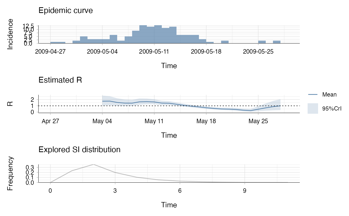 ## the second plot produced shows, at each each day,
## the estimate of the reproduction number
## over the 7-day window finishing on that day.
if (FALSE) { # \dontrun{
## Note the following examples use an MCMC routine
## to estimate the serial interval distribution from data,
## so they may take a few minutes to run
## estimate the reproduction number (method "si_from_data")
res <- estimate_R(
Flu2009$incidence,
method = "si_from_data",
si_data = Flu2009$si_data,
config = make_config(list(
mcmc_control = make_mcmc_control(list(burnin = 1000, thin = 10, seed = 1)),
n1 = 1000,
n2 = 50,
si_parametric_distr = "G"
))
)
plot(res)
## the second plot produced shows, at each each day,
## the estimate of the reproduction number
## over the 7-day window finishing on that day.
} # }
## the second plot produced shows, at each each day,
## the estimate of the reproduction number
## over the 7-day window finishing on that day.
if (FALSE) { # \dontrun{
## Note the following examples use an MCMC routine
## to estimate the serial interval distribution from data,
## so they may take a few minutes to run
## estimate the reproduction number (method "si_from_data")
res <- estimate_R(
Flu2009$incidence,
method = "si_from_data",
si_data = Flu2009$si_data,
config = make_config(list(
mcmc_control = make_mcmc_control(list(burnin = 1000, thin = 10, seed = 1)),
n1 = 1000,
n2 = 50,
si_parametric_distr = "G"
))
)
plot(res)
## the second plot produced shows, at each each day,
## the estimate of the reproduction number
## over the 7-day window finishing on that day.
} # }