An introduction to odin2 and dust2

odin

• A “domain specific language”
• Originally designed for ordinary differential equations
• Some very basic discrete time/stochastic support

Odin is a DSL - a domain specific language. It exists to describe a specific problem efficiently. We developed it to describe ordinary differential equations which evolve a system in continuous time. This is a great target for DSL because it’s just a collection of mathematical truths - rates exist independent of any idea of order of operation.

odin

library(odin2)
library(dust2)
library(monty)

ODE models

deriv(S) <- -beta * S * I / N
deriv(I) <- beta * S * I / N - gamma * I
deriv(R) <- gamma * I

initial(S) <- N - I0
initial(I) <- I0
initial(R) <- 0

N <- parameter(1000)
I0 <- parameter(10)
beta <- parameter(0.2)
gamma <- parameter(0.1)

\[\begin{gather*} \frac{dS}{dt} = -\beta S \frac{I}{N}\\ \frac{dI}{dt} = \beta S \frac{I}{N} - \gamma I\\ \frac{dR}{dt} = \gamma I \end{gather*}\]

Things to note:

• out of order definition
• every variable has initial and deriv pair

Compiling the model with odin2

sir_ode <- odin({
  deriv(S) <- -beta * S * I / N
  deriv(I) <- beta * S * I / N - gamma * I
  deriv(R) <- gamma * I
  
  initial(S) <- N - I0
  initial(I) <- I0
  initial(R) <- 0
  
  N <- parameter(1000)
  I0 <- parameter(10)
  beta <- parameter(0.2)
  gamma <- parameter(0.1)
})

The odin call generates C code, compiles it with gcc or clang to create a shared library, and loads that plus support code into R to create a generator object gen

Running the model with dust2

sys <- dust_system_create(sir_ode, pars = list())
dust_system_set_state_initial(sys)
t <- seq(0, 100)
y <- dust_system_simulate(sys, t)

The output has dimensions number of states x number of timepoints

dim(y)
#> [1]   3 101

Unpacking states

Output can be nicely unpacked into the different states using dust_unpack_state

y <- dust_unpack_state(sys, y)

plot(t, y$I, type = "l", xlab = "Time", ylab = "I")

From the generator object gen we can construct a model (mod), here using no parameters – just using default parameters as defined above. We run over a set of times and output the value of the system at a number of intermediate times.

Stochastic models

update(S) <- S - n_SI
update(I) <- I + n_SI - n_IR
update(R) <- R + n_IR

initial(S) <- N - I0
initial(I) <- I0
initial(R) <- 0

p_SI <- 1 - exp(-beta * I / N * dt)
p_IR <- 1 - exp(-gamma * dt)
n_SI <- Binomial(S, p_SI)
n_IR <- Binomial(I, p_IR)

N <- parameter(1000)
I0 <- parameter(10)
beta <- parameter(0.2)
gamma <- parameter(0.1)

\[\begin{gather*} S(t + \Delta t) = S(t) - n_{SI}\\ I(t + \Delta t) = I(t) + n_{SI} - n_{IR}\\ R(t + \Delta t) = R(t) + n_{IR} \end{gather*}\]

• dt is a special parameter
• every variable has initial and update pair

…compared with ODE models

update(S) <- S - n_SI
update(I) <- I + n_SI - n_IR
update(R) <- R + n_IR

initial(S) <- N - I0
initial(I) <- I0
initial(R) <- 0

p_SI <- 1 - exp(-beta * I / N * dt)
p_IR <- 1 - exp(-gamma * dt)
n_SI <- Binomial(S, p_SI)
n_IR <- Binomial(I, p_IR)

N <- parameter(1000)
I0 <- parameter(10)
beta <- parameter(0.2)
gamma <- parameter(0.1)

deriv(S) <- -beta * S * I / N
deriv(I) <- beta * S * I / N - gamma * I
deriv(R) <- gamma * I

initial(S) <- N - I0
initial(I) <- I0
initial(R) <- 0

N <- parameter(1000)
I0 <- parameter(10)
beta <- parameter(0.2)
gamma <- parameter(0.1)

Compiling with odin2

sir <- odin({
  update(S) <- S - n_SI
  update(I) <- I + n_SI - n_IR
  update(R) <- R + n_IR
  
  initial(S) <- N - I0
  initial(I) <- I0
  initial(R) <- 0
  
  p_SI <- 1 - exp(-beta * I / N * dt)
  p_IR <- 1 - exp(-gamma * dt)
  n_SI <- Binomial(S, p_SI)
  n_IR <- Binomial(I, p_IR)
  
  N <- parameter(1000)
  I0 <- parameter(10)
  beta <- parameter(0.2)
  gamma <- parameter(0.1)
})

Running a single simulation

sys <- dust_system_create(sir, pars = list(), dt = 0.25)
dust_system_set_state_initial(sys)
t <- seq(0, 100)
y <- dust_system_simulate(sys, t)
y <- dust_unpack_state(sys, y)

plot(t, y$I, type = "l", xlab = "Time", ylab = "Infected population")

Running multiple simulations

sys <- dust_system_create(sir, pars = list(), n_particles = 50,
                                 dt = 0.25)
dust_system_set_state_initial(sys)
t <- seq(0, 100)
y <- dust_system_simulate(sys, t)
y <- dust_unpack_state(sys, y)
matplot(t, t(y$I), type = "l", lty = 1, col = "#00000044",
        xlab = "Time", ylab = "Infected population")

Calculating incidence with zero_every

sir <- odin({
  update(S) <- S - n_SI
  update(I) <- I + n_SI - n_IR
  update(R) <- R + n_IR
  update(incidence) <- incidence + n_SI
  
  p_SI <- 1 - exp(-beta * I / N * dt)
  p_IR <- 1 - exp(-gamma * dt)
  n_SI <- Binomial(S, p_SI)
  n_IR <- Binomial(I, p_IR)
  
  initial(S) <- N - I0
  initial(I) <- I0
  initial(R) <- 0
  initial(incidence, zero_every = 1) <- 0
  
  N <- parameter(1000)
  I0 <- parameter(10)
  beta <- parameter(0.2)
  gamma <- parameter(0.1)
})

Incidence accumulates then resets

sys <- dust_system_create(sir, pars = list(), dt = 1 / 128)
dust_system_set_state_initial(sys)
t <- seq(0, 20, by = 1 / 128)
y <- dust_system_simulate(sys, t)
y <- dust_unpack_state(sys, y)

plot(t[t %% 1 == 0], y$incidence[t %% 1 == 0], type = "o", pch = 19,
     ylab = "Infection incidence", xlab = "Time")
lines(t, y$incidence, col = "red")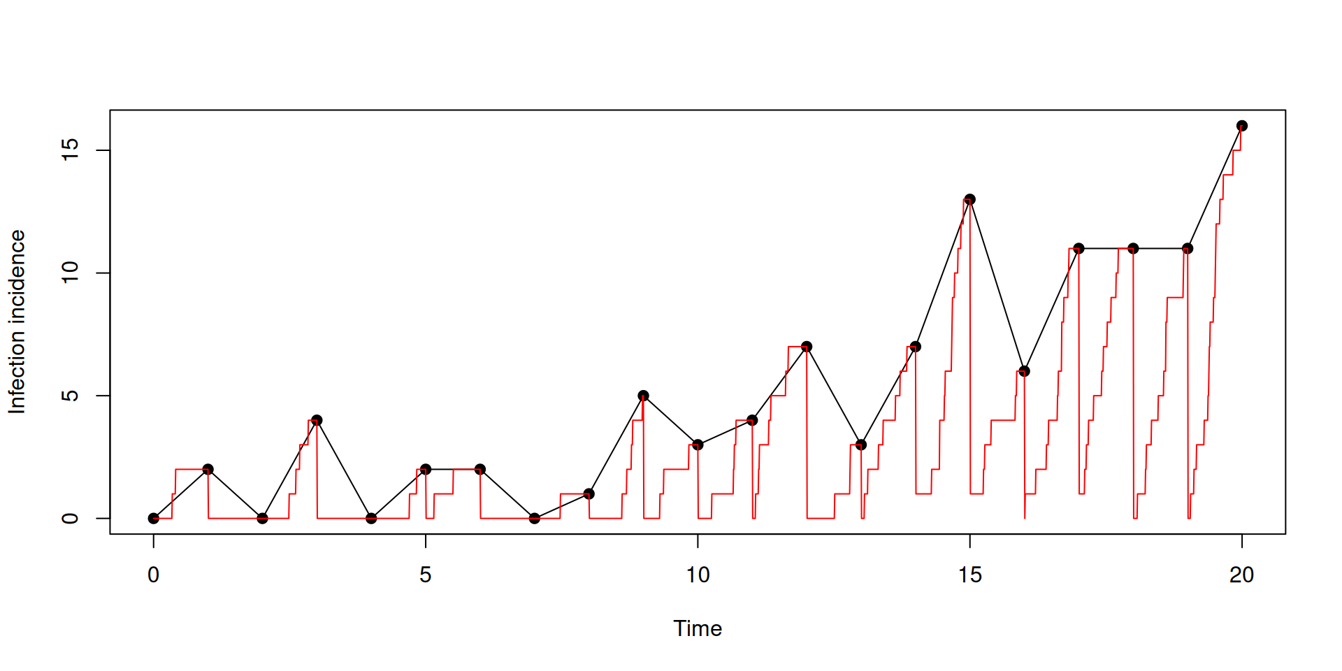

Time-varying inputs: using time

sir <- odin({
  update(S) <- S - n_SI
  update(I) <- I + n_SI - n_IR
  update(R) <- R + n_IR
  update(incidence) <- incidence + n_SI
  
  seed <- if (time == seed_time) seed_size else 0
  
  p_SI <- 1 - exp(-beta * I / N * dt)
  p_IR <- 1 - exp(-gamma * dt)
  n_SI <- min(seed + Binomial(S, p_SI), S)
  n_IR <- Binomial(I, p_IR)
  
  initial(S) <- N
  initial(I) <- 0
  initial(R) <- 0
  initial(incidence, zero_every = 1) <- 0
  
  N <- parameter(1000)
  beta <- parameter(0.2)
  gamma <- parameter(0.1)
  seed_time <- parameter()
  seed_size <- parameter()
})

Time-varying inputs: using time

pars <- list(seed_time = 10, seed_size = 15)
sys <- dust_system_create(sir, pars = pars, dt = 0.25)
dust_system_set_state_initial(sys)
t <- seq(0, 100)
y <- dust_system_simulate(sys, t)
y <- dust_unpack_state(sys, y)

plot(t, y$I, type = "l", xlab = "Time", ylab = "Infected population")

Time-varying inputs: using interpolate

The interpolate function in odin can be used for time-varying parameters, with specification of

• the times of changepoints
• the values at those changepoints
• the type of interpolation: linear, constant or spline

Time-varying inputs: using interpolate

sir <- odin({
  update(S) <- S - n_SI
  update(I) <- I + n_SI - n_IR
  update(R) <- R + n_IR
  update(incidence) <- incidence + n_SI
  
  beta <- interpolate(beta_time, beta_value, "constant")
  beta_time <- parameter()
  beta_value <- parameter()
  dim(beta_time, beta_value) <- parameter(rank = 1)
  
  p_SI <- 1 - exp(-beta * I / N * dt)
  p_IR <- 1 - exp(-gamma * dt)
  n_SI <- Binomial(S, p_SI)
  n_IR <- Binomial(I, p_IR)
  
  initial(S) <- N - I0
  initial(I) <- I0
  initial(R) <- 0
  initial(incidence, zero_every = 1) <- 0
  
  N <- parameter(1000)
  I0 <- parameter(10)
  gamma <- parameter(0.1)
})

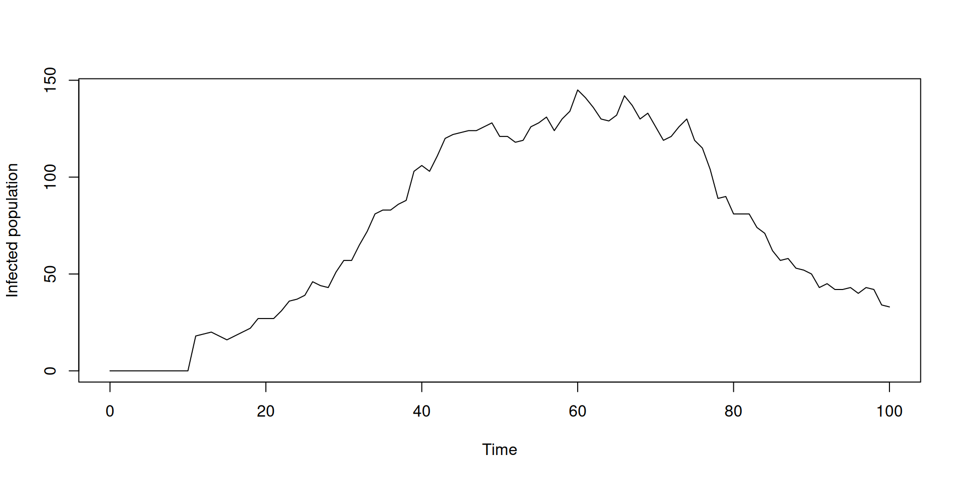
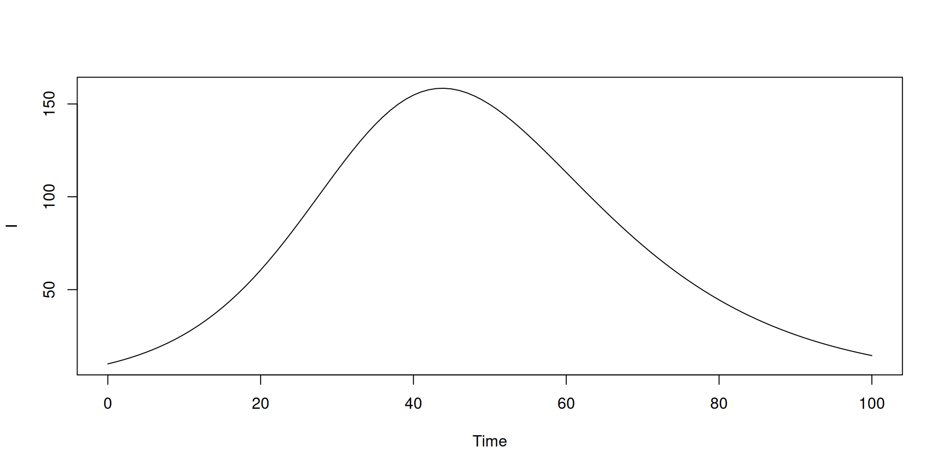
Time-varying inputs: using interpolate

pars <- list(beta_time = c(0, 30), beta_value = c(0.2, 1))
sys <- dust_system_create(sir, pars = pars, dt = 0.25)
dust_system_set_state_initial(sys)
t <- seq(0, 100)
y <- dust_system_simulate(sys, t)
y <- dust_unpack_state(sys, y)

plot(t, y$I, type = "l", xlab = "Time", ylab = "Infected population")
abline(v = 30, lty = 3)

Using arrays

sir_age <- odin({
  # Equations for transitions between compartments by age group
  update(S[]) <- S[i] - n_SI[i]
  update(I[]) <- I[i] + n_SI[i] - n_IR[i]
  update(R[]) <- R[i] + n_IR[i]
  update(incidence) <- incidence + sum(n_SI)
  
  # Individual probabilities of transition:
  p_SI[] <- 1 - exp(-lambda[i] * dt) # S to I
  p_IR <- 1 - exp(-gamma * dt) # I to R
  
  # Calculate force of infection
  
  # age-structured contact matrix: m[i, j] is mean number
  # of contacts an individual in group i has with an
  # individual in group j per time unit
  m <- parameter()
  
  # here s_ij[i, j] gives the mean number of contacts an
  # individual in group i will have with the currently
  # infectious individuals of group j
  s_ij[, ] <- m[i, j] * I[j]
  
  # lambda[i] is the total force of infection on an
  # individual in group i
  lambda[] <- beta * sum(s_ij[i, ])
  
  # Draws from binomial distributions for numbers
  # changing between compartments:
  n_SI[] <- Binomial(S[i], p_SI[i])
  n_IR[] <- Binomial(I[i], p_IR)
  
  initial(S[]) <- S0[i]
  initial(I[]) <- I0[i]
  initial(R[]) <- 0
  initial(incidence, zero_every = 1) <- 0
  
  S0 <- parameter()
  I0 <- parameter()
  beta <- parameter(0.2)
  gamma <- parameter(0.1)
  
  n_age <- parameter()
  dim(S, S0, n_SI, p_SI) <- n_age
  dim(I, I0, n_IR) <- n_age
  dim(R) <- n_age
  dim(m, s_ij) <- c(n_age, n_age)
  dim(lambda) <- n_age
})

Using arrays

pars <- list(S0 = c(990, 1000),
             I0 = c(10, 0),
             m = matrix(c(1.8, 0.4, 0.4, 1.2) / 2000, 2, 2),
             beta = 0.2,
             gamma = 0.1,
             n_age = 2)

Remember: m[i, j] is the mean number of contacts per time unit for an individual in group i has with an individual in group j

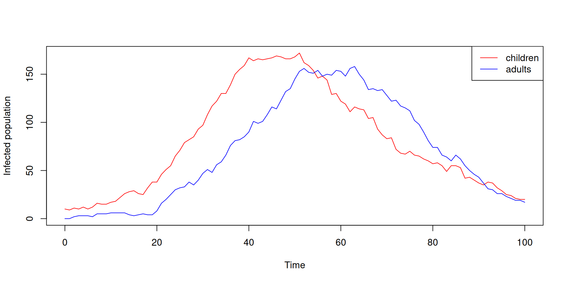
Using arrays

sys <- dust_system_create(sir_age, pars = pars, dt = 0.25)
dust_system_set_state_initial(sys)
t <- seq(0, 100)
y <- dust_system_simulate(sys, t)
y <- dust_unpack_state(sys, y)

matplot(t, t(y$I), type = "l", lty = 1, col = c("red", "blue"),
        xlab = "Time", ylab = "Infected population")
legend("topright", c("children", "adults"), col = c("red", "blue"), lty = 1)

Key features of arrays

• All arrays (whether state variable or parameter) need a dim equation
• No use of i, j etc on LHS - indexing on the LHS is implicit
• Support for up to 8 dimensions, with index variables i, j, k, l, i5, i6, i7, i8
• Functions for reducing arrays such as sum, prod, min, max - can be applied over entire array or slices

Arrays: model with age and vaccine

sir_age_vax <- odin({
  # Equations for transitions between compartments by age group
  update(S[, ]) <- new_S[i, j]
  update(I[, ]) <- I[i, j] + n_SI[i, j] - n_IR[i, j]
  update(R[, ]) <- R[i, j] + n_IR[i, j]
  update(incidence) <- incidence + sum(n_SI)
  
  # Individual probabilities of transition:
  p_SI[, ] <- 1 - exp(-rel_susceptibility[j] * lambda[i] * dt) # S to I
  p_IR <- 1 - exp(-gamma * dt) # I to R
  p_vax[, ] <- 1 - exp(-eta[i, j] * dt)
  
  # Force of infection
  m <- parameter() # age-structured contact matrix
  s_ij[, ] <- m[i, j] * sum(I[j, ])
  lambda[] <- beta * sum(s_ij[i, ])
  
  # Draws from binomial distributions for numbers changing between
  # compartments:
  n_SI[, ] <- Binomial(S[i, j], p_SI[i, j])
  n_IR[, ] <- Binomial(I[i, j], p_IR)
  
  # Nested binomial draw for vaccination in S
  # Assume you cannot move vaccine class and get infected in same step
  n_S_vax[, ] <- Binomial(S[i, j] - n_SI[i, j], p_vax[i, j])
  new_S[, 1] <- S[i, j] - n_SI[i, j] - n_S_vax[i, j] + n_S_vax[i, n_vax]
  new_S[, 2:n_vax] <- S[i, j] - n_SI[i, j] - n_S_vax[i, j] + n_S_vax[i, j - 1]
  
  initial(S[, ]) <- S0[i, j]
  initial(I[, ]) <- I0[i, j]
  initial(R[, ]) <- 0
  initial(incidence, zero_every = 1) <- 0
  
  # User defined parameters - default in parentheses:
  S0 <- parameter()
  I0 <- parameter()
  beta <- parameter(0.0165)
  gamma <- parameter(0.1)
  eta <- parameter()
  rel_susceptibility <- parameter()
  
  # Dimensions of arrays
  n_age <- parameter()
  n_vax <- parameter()
  dim(S, S0, n_SI, p_SI) <- c(n_age, n_vax)
  dim(I, I0, n_IR) <- c(n_age, n_vax)
  dim(R) <- c(n_age, n_vax)
  dim(m, s_ij) <- c(n_age, n_age)
  dim(lambda) <- n_age
  dim(eta) <- c(n_age, n_vax)
  dim(rel_susceptibility) <- c(n_vax)
  dim(p_vax, n_S_vax, new_S) <- c(n_age, n_vax)
})

Arrays: boundary conditions

Multiline equations can be used to deal with boundary conditions, e.g. we have

new_S[, 1] <- S[i, j] - n_SI[i, j] - n_S_vax[i, j] + n_S_vax[i, n_vax]
new_S[, 2:n_vax] <- S[i, j] - n_SI[i, j] - n_S_vax[i, j] + n_S_vax[i, j - 1]

which we could also write as

new_S[, ] <- S[i, j] - n_SI[i, j] - n_S_vax[i, j]
new_S[, 1] <- new_S[i, j] + n_S_vax[i, n_vax]
new_S[, 2:n_vax] <- new_S[i, j] + n_S_vax[i, j - 1]

or another way of writing this would be to use if else

new_S[, ] <- S[i, j] - n_SI[i, j] - n_S_vax[i, j] +
    (if (j == 1) n_S_vax[i, n_vax] else n_S_vax[i, j - 1])