Future of the tools

What is new?

• Since odin v1 (classic odin, pre 2020)
  • comparison to data and likelihood support
  • run multiple sets of parameters at once
  • run in parallel

What is new?

• Since odin.dust (2024 rewrite)
  • more efficient parameter updating
  • parameter packers
  • better parallelism
  • periodic variable resetting (zero_every)
  • better error messages
  • compile time array bounds checking
  • debugging support

Syntax changes

• user() -> parameter()
• Discrete models have a proper time basis, dt is now a reserved word
• No longer use R’s names for distribution functions
• Named arguments allow clearer code

Automatic migration

sys <- odin2::odin({
  update(y) <- y + rnorm(0, sd)
  initial(y) <- 0
  sd <- user()
})

Warning in odin2::odin({: Found 2 compatibility issues
Replace calls to 'user()' with 'parameter()'
✖ sd <- user()
✔ sd <- parameter()
Replace calls to r-style random number calls (e.g., 'rnorm()') with monty-stye
calls (e.g., 'Normal()')
✖ update(y) <- y + rnorm(0, sd)
✔ update(y) <- y + Normal(0, sd)

You can use odin_migrate() to rewrite code.

Limitations

• Much slower compilation time (we will mitigate this by using js)
• Delays less flexible than in version 1 (cannot be used in discrete time models, the default argument has been removed)

Practical considerations

• Handful of missing features from odin v1 and dust v1 (odin.dust)
  • delayed delays
  • mixed time models
  • compilation to JavaScript
  • extendable via C++

Practical considerations

• The great package migration
  • dust2 to dust
  • odin2 to odin and all onto CRAN
  • Once on CRAN, our ability to change the dust and monty C++ code is reduced

Planned new features

GPU support

• Massively parallel stochastic models
  • Proof-of-concept: 1 consumer GPU = 5-10 32-core nodes
• Simulation with many parameter sets harder

MPI/HPC support

• Alternative approach to parallelism
  • based on message passing, rather than shared memory
• Use CPU-based HPC with fast networking
• We are interested in hearing about models that can take advantage of these levels of parallelism

More radical changes to the DSL?

• Support for events
• More bounds checking and debugging support
• Vector-returning functions (multinomial, matrix mutiplication, etc)
• Describe models in terms of flows
• Composable sub models (I am told this is very hard!)
• Improve monty’s little DSL!
• What else?

Improvement of supported particle methods?

• SMC^2, IF^2
• PF other than bootstrap
• Methods based on estimates of ratio of density rather than ratio of density estimates

Automatic differentiation

Gradient vs random walk

• Goal: Sample from the posterior efficiently
• 🐢 Random Walk MCMC:
  • No knowledge of shape of posterior
  • Can get stuck in tight or curved regions
• ⚡ Gradient-based methods:
  • Use the local slope to move efficiently
  • Better scaling in high dimensions

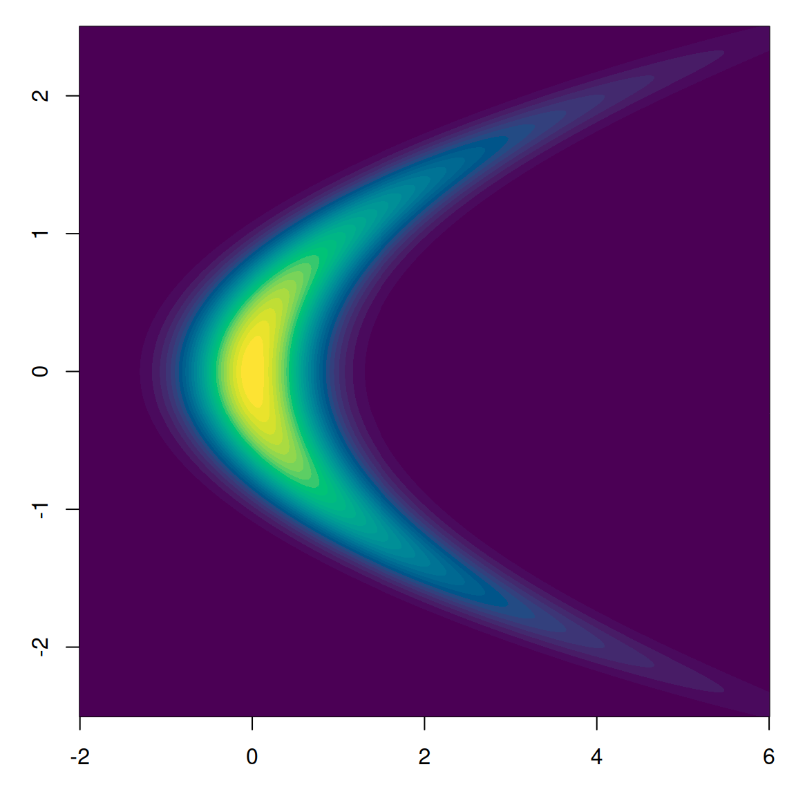
🍌 The Banana Problem

library(monty)
m <- monty_example("banana", sigma = 0.5)

a <- seq(-2, 6, length.out = 1000)
b <- seq(-2.5, 2.5, length.out = 1000)
z <- outer(a, b, function(alpha, beta) {
  exp(monty_model_density(m, rbind(alpha, beta)))
})

• This posterior has a strong nonlinear correlation
• Random walk proposals struggle to explore this space

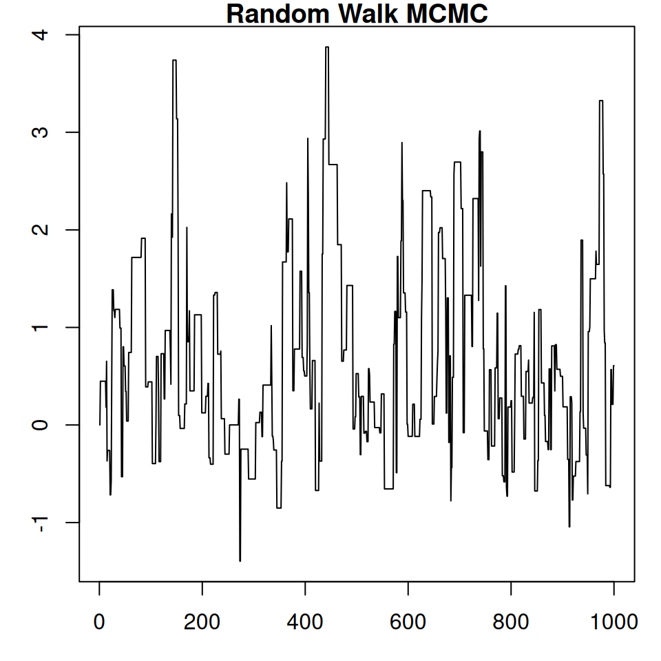
🐢 Random Walk MCMC: Limitation

set.seed(42)
sampler_rw <- monty_sampler_random_walk(vcv = diag(2)*1.5)
samples_rw <- monty_sample(m, sampler_rw, n_steps = 1000, initial = c(0,0))

⡀⠀ Sampling  ■                                |   0% ETA:  3s

✔ Sampled 1000 steps across 1 chain in 41ms

• Acceptance rate 0.236
• Small steps to avoid rejection → slow mixing
• Misses curved geometry
• Inefficient in higher dimensions

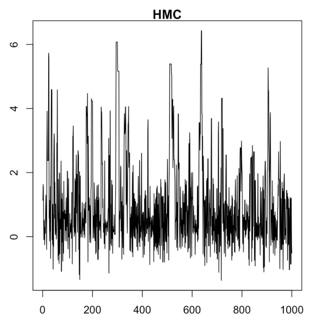
⚡ Gradient-Based: Faster & Smarter

sampler_hmc <- monty_sampler_hmc(epsilon = 0.2, n_integration_steps = 10)
# samples_hmc <- monty_sample(m, sampler_hmc, n_steps = 1000, initial = c(0,0))

• Acceptance rate 0.236
• Uses gradient of the log posterior
• Efficiently explores curved shapes
• Much better mixing in fewer steps
• But potentially expensive to compute gradients

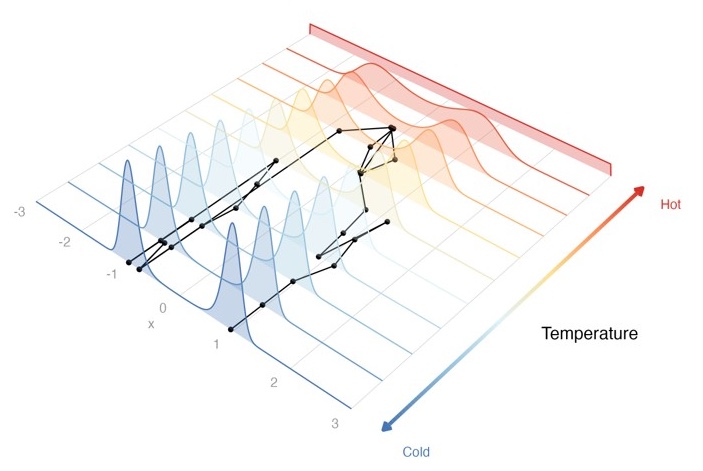
Reverse AutoDiff in odin

• Think of your model as a computational graph: data + parameters → output
• Reverse AD walks backward through this graph to efficiently compute gradients
• ✅ More accurate than numerical methods
• ✅ Much faster (especially in high dimensions)

🛠 In odin, you write the model normally — gradients come for free

✅ Summary

• Gradient-based methods like HMC/NUTS:
  • Are more efficient, especially for complex or high-dimensional posteriors
  • Adapt to local geometry (no tuning random walk scale!)
  • Often yield better convergence diagnostics
• 🚀 For users fitting models: you’ll get faster, more reliable inference with gradients when available!

🗺️ Autodiff roadmap

• Simple support implemented as a proof-of-concept
  • deterministic discrete time models with no arrays
• Expand to support ODE models, models with arrays
• Fully implement algorithms in monty that can exploit gradients
  • HMC, NUTS, variational inference

Parallel tempering