Fitting odin models with monty
A pragmatic introduction
On your laptop:
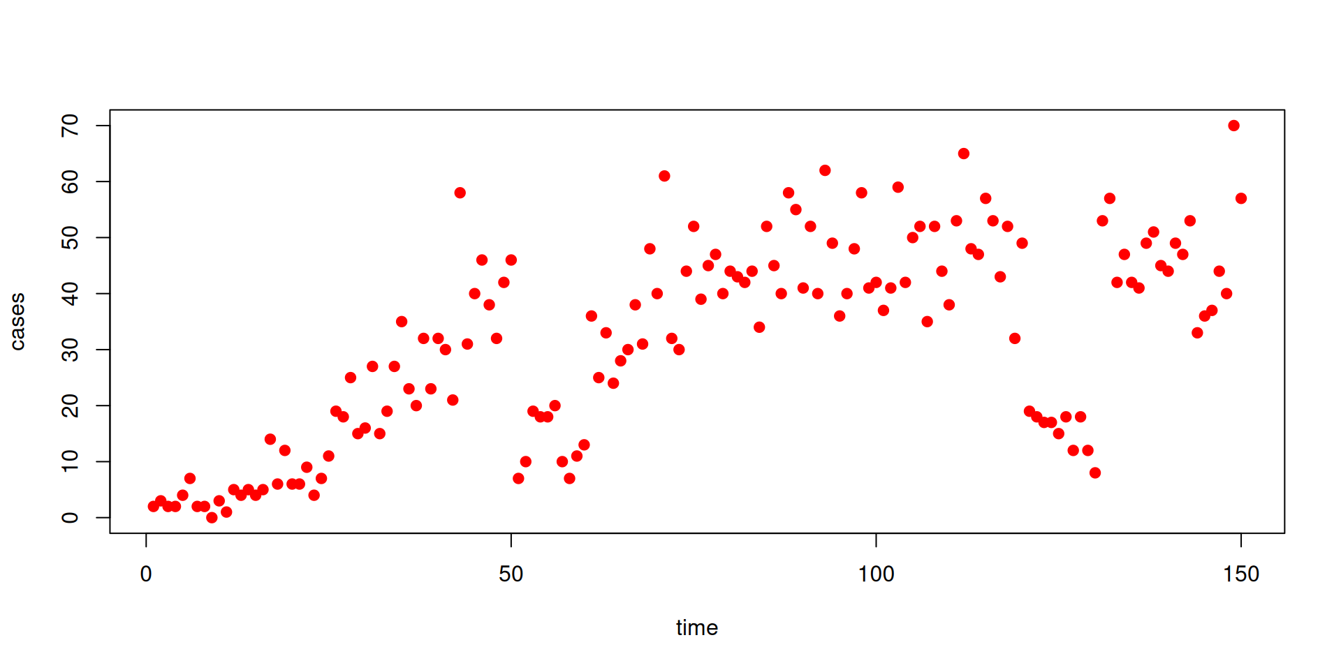
The data
Calculating likelihood: particle filtering
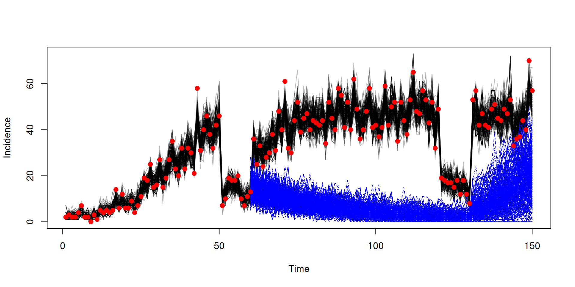
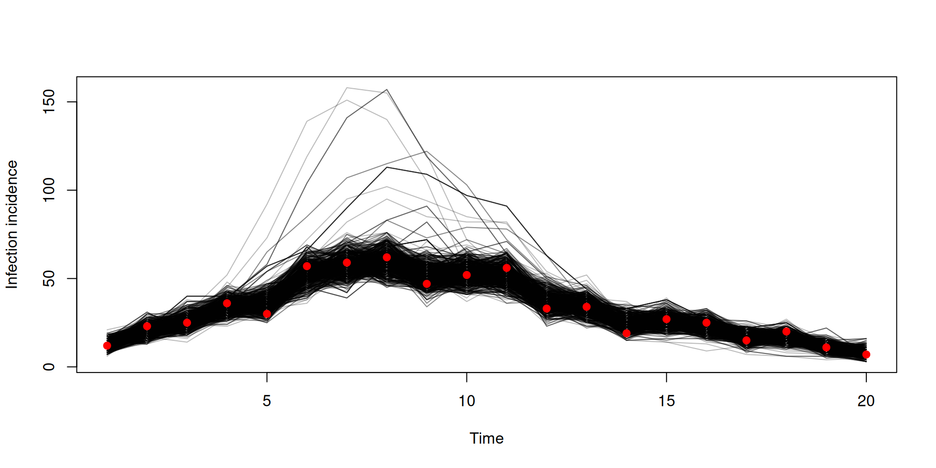
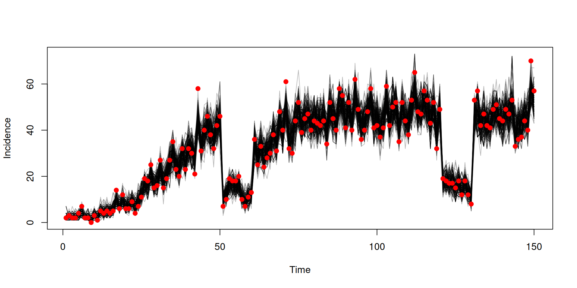
Filtered trajectories
dust_likelihood_run(filter, list(beta = 0.4, gamma = 0.2),
                    save_trajectories = TRUE)
#> [1] -87.92554
y <- dust_likelihood_last_trajectories(filter)
y <- dust_unpack_state(filter, y)
matplot(data$time, t(y$incidence), type = "l", col = "#00000044", lty = 1,
        xlab = "Time", ylab = "Incidence")
points(data, pch = 19, col = "red")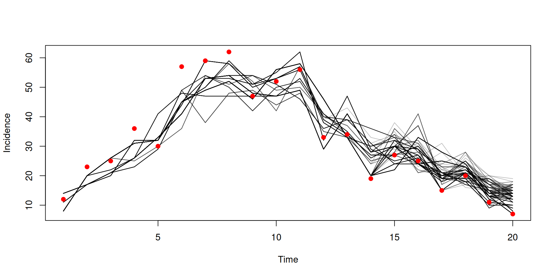
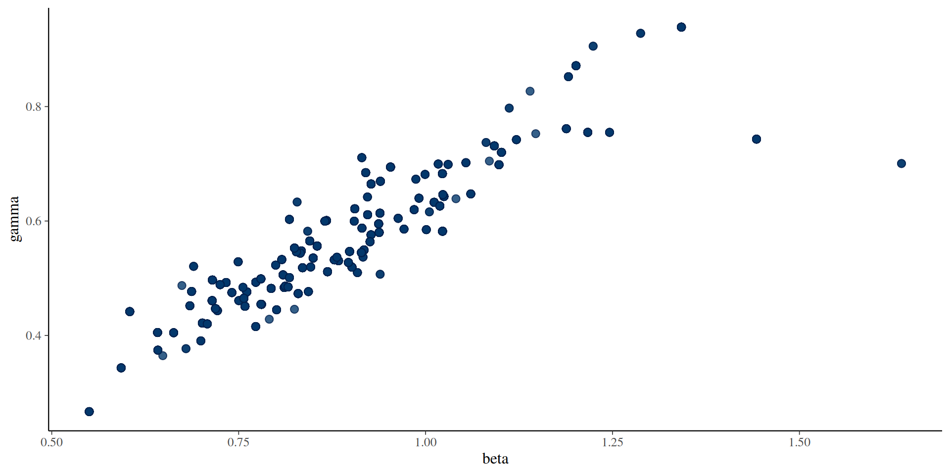
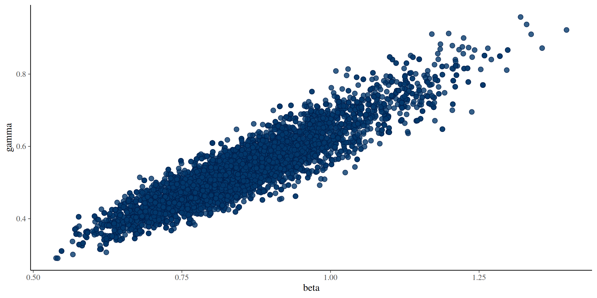
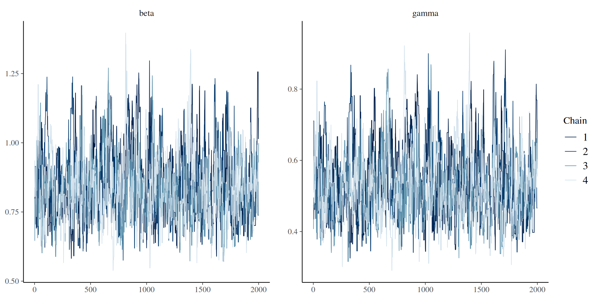
The results: parameters
You can use the posterior package in conjunction with bayesplot (and then also ggplot2)
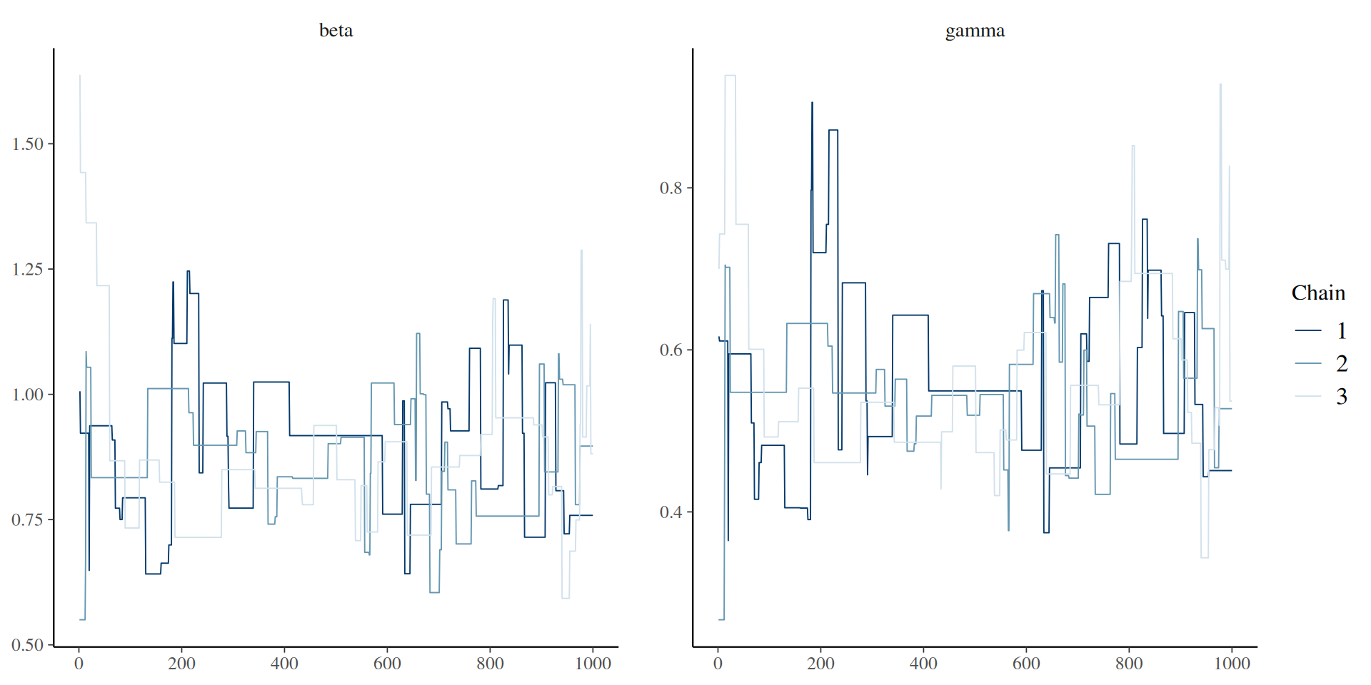
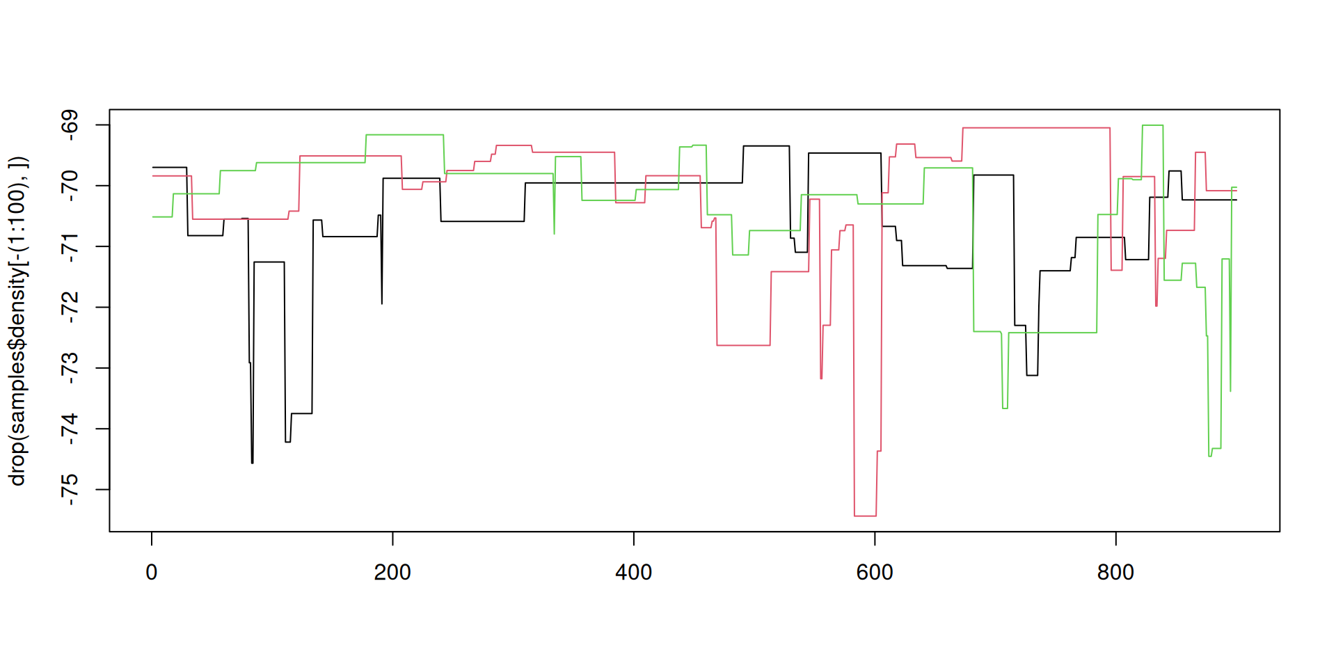
The result: traceplots
The result: density over time
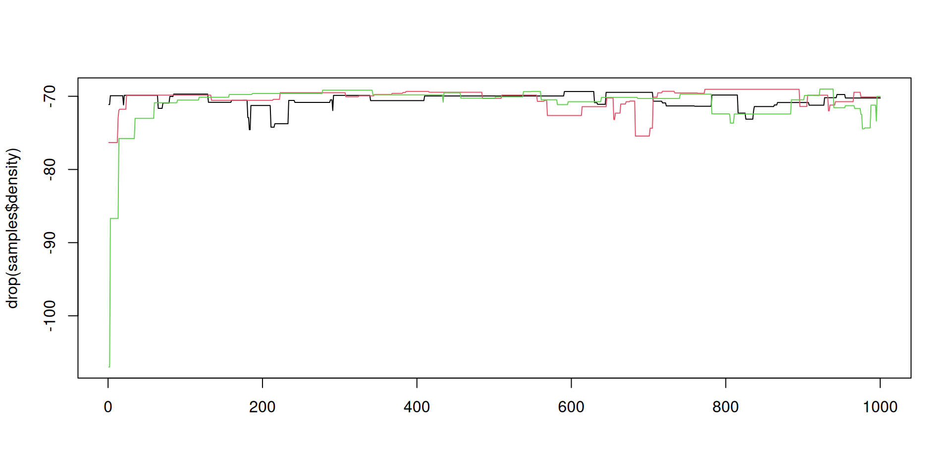
The result: density over time
Better mixing
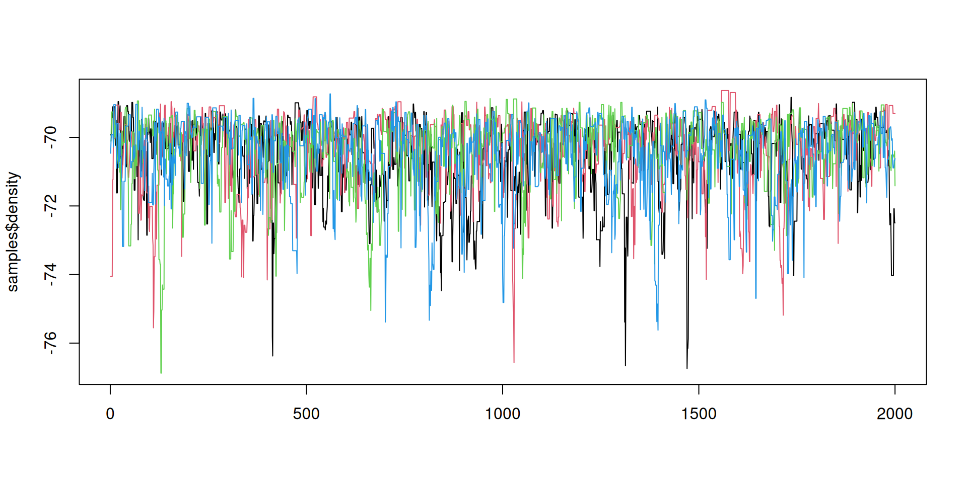
Better mixing: the results
Better mixing: the results
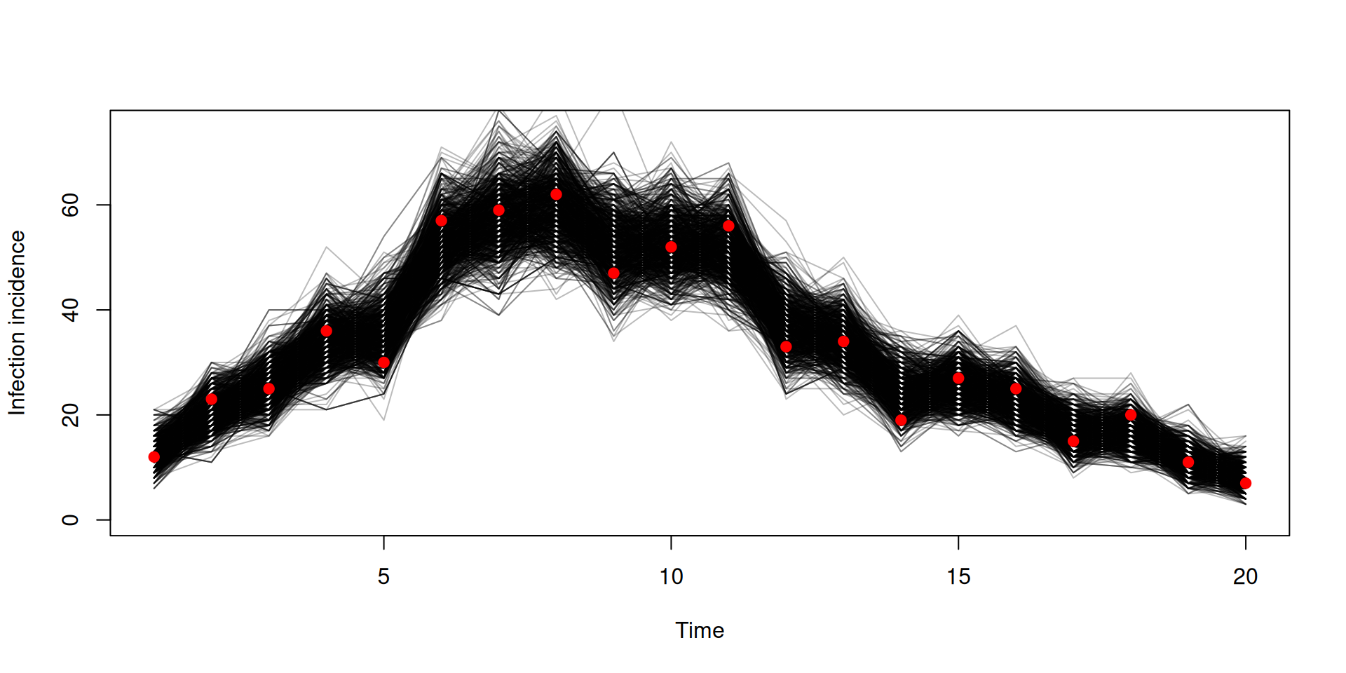
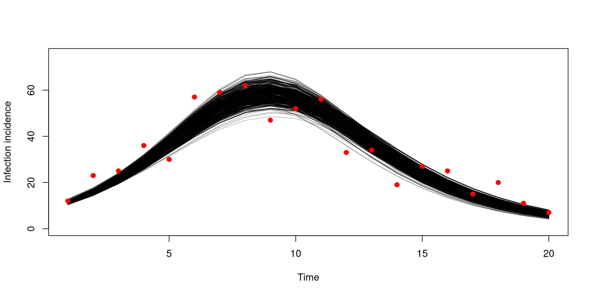
Trajectories
Stochastic v deterministic comparison
Stochastic v deterministic comparison
Stochastic v deterministic comparison
pars_stochastic <- array(samples$pars, c(2, 500))
pars_deterministic <- array(samples_det$pars, c(2, 500))
plot(pars_stochastic[1, ], pars_stochastic[2, ], ylab = "gamma", xlab = "beta",
     pch = 19, col = "blue")
points(pars_deterministic[1, ], pars_deterministic[2, ], pch = 19, col = "red")
legend("bottomright", c("stochastic fit", "deterministic fit"), pch = c(19, 19),
       col = c("blue", "red"))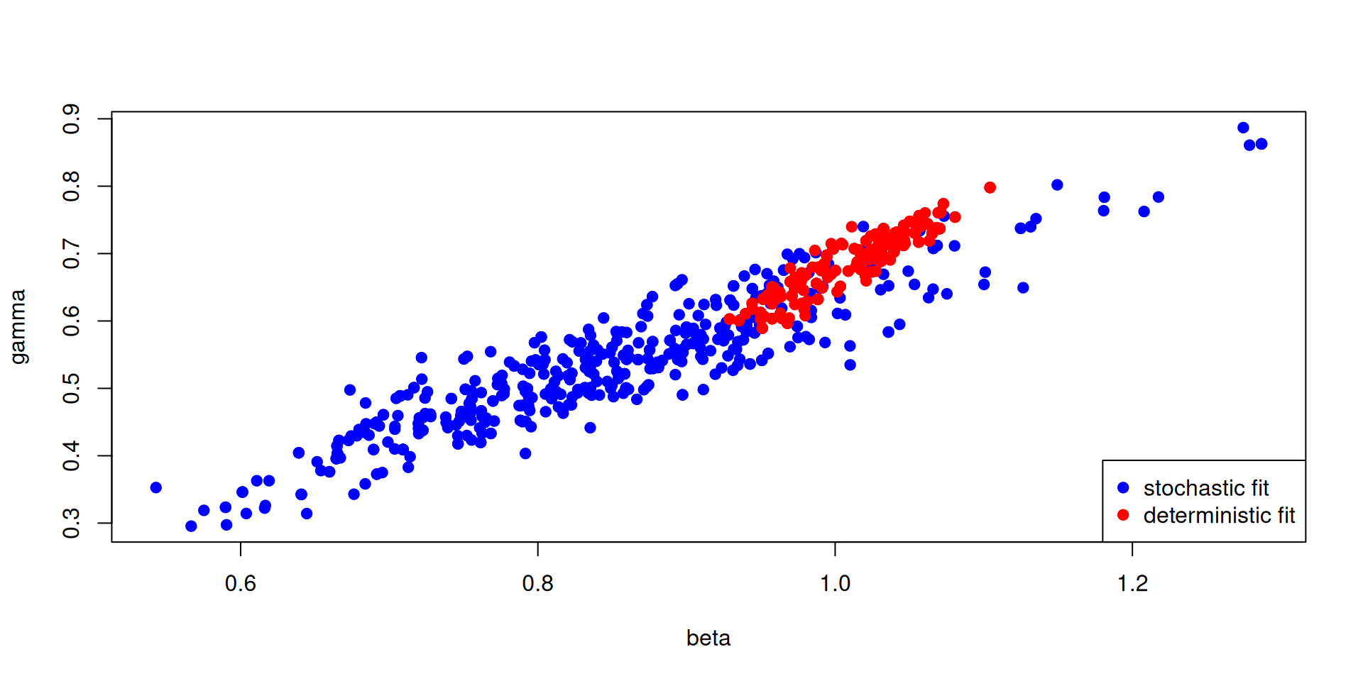
Projections and counterfactuals
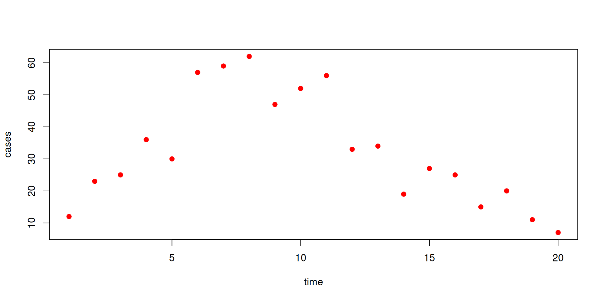
Let’s use some new data
Fit to data
Running projection using the end state
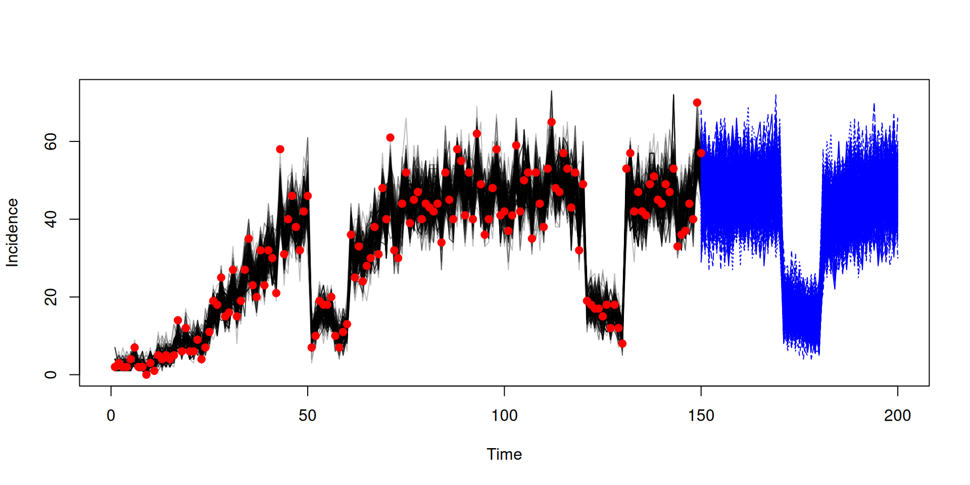
Running counterfactual using the snapshot